Documentation
3934 Time-Waveform & Spectrum
MS-3934: Vibration Analysis Studio iPadOS® version
- Version: 1.49 (b.126)
- Author: D. Bukowitz
- Created: 04 Mar, 2021
- Update: 21 Nov, 2022
If you have any questions that are beyond the scope of this document, Please feel free to email via info@sens-os.com
Description
These 3 modules will allow the user to display:
There are multiple options for each module to display cursors, an integrated or double-integrated spectrum, windowing, filtering, cut-off filter, etc
Compatibility
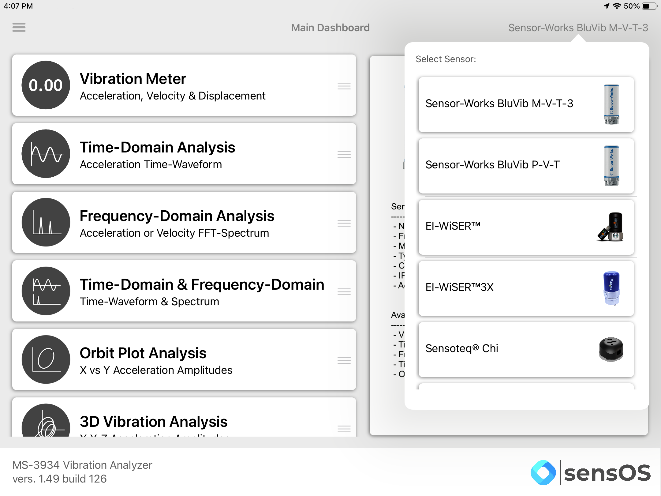
These modules are compatible with the following sensors:
- SensorWorks BluVib P-V-T (1 Axis)
- SensorWorks BluVib M-V-T-3 (3 Axis)
- EI-WiSER™3X (3 Axis)
- Sensoteq® Chi (3 Axis)
- Digiducer (1 Axis)
- Digital ICP Signal Conditiones (2 Axis)
- CTC WA102-1A (1 Axis)
- EI-Wiser™ (2 Axis)
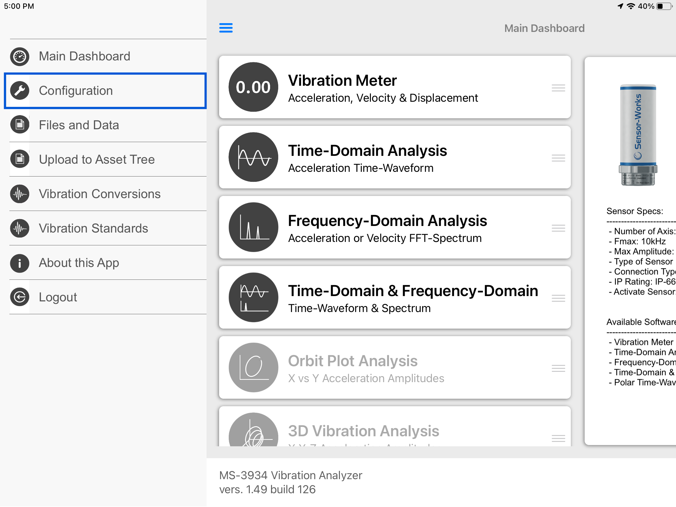
Main Menu
- Tap on the Sensor name button to open the list of available sensors, and select the sensor type from the list
- Select any of the three following modules:
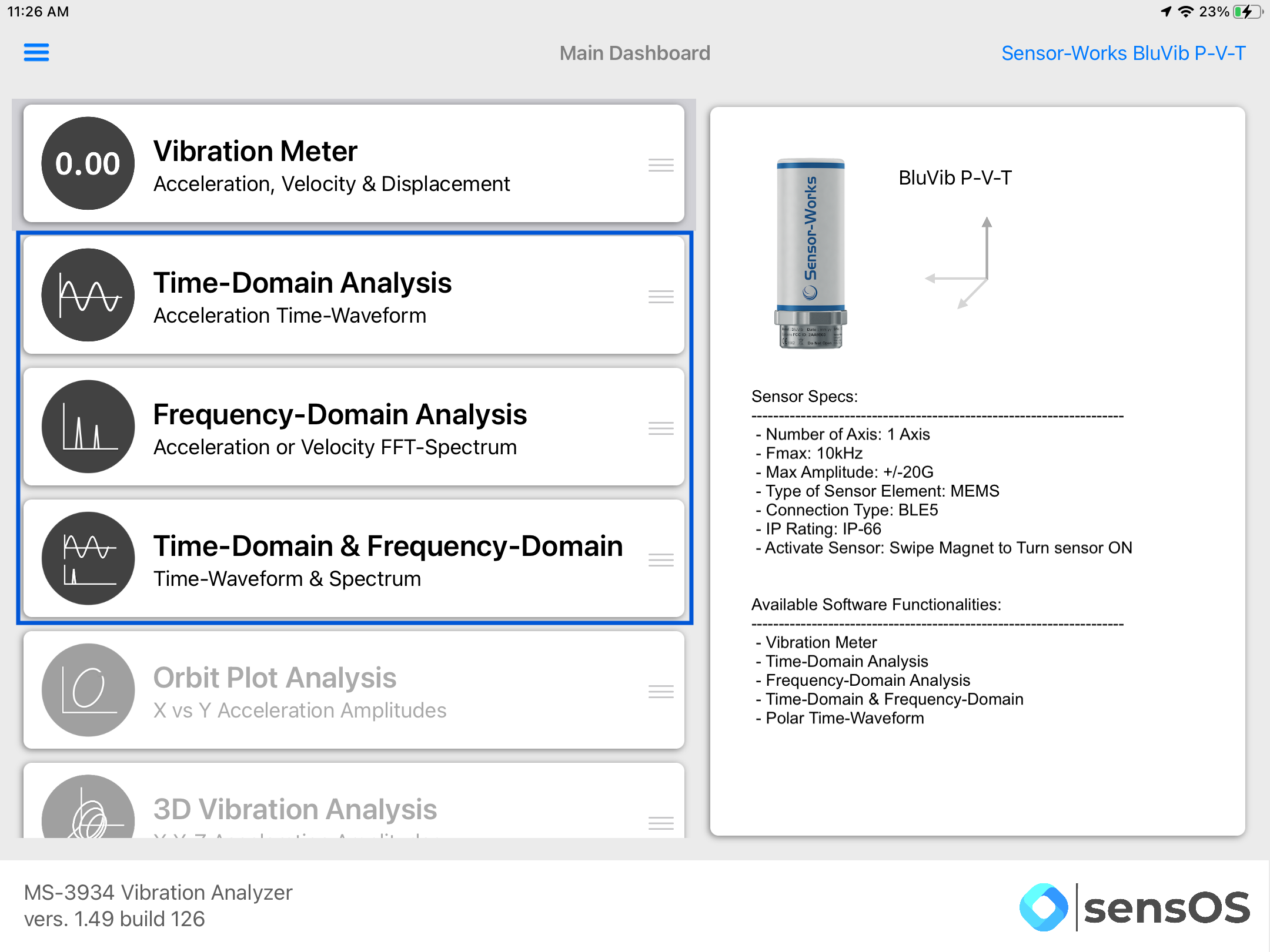
Note: The user can change the order of the functionalities in the list by dragging it from the right button on each cell
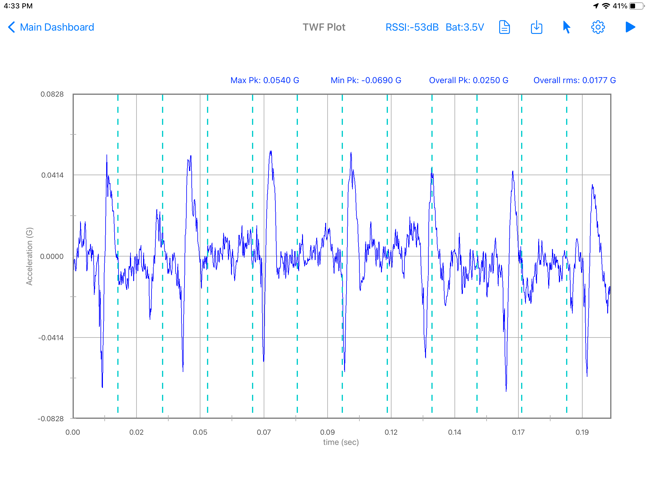
Time-Waveform
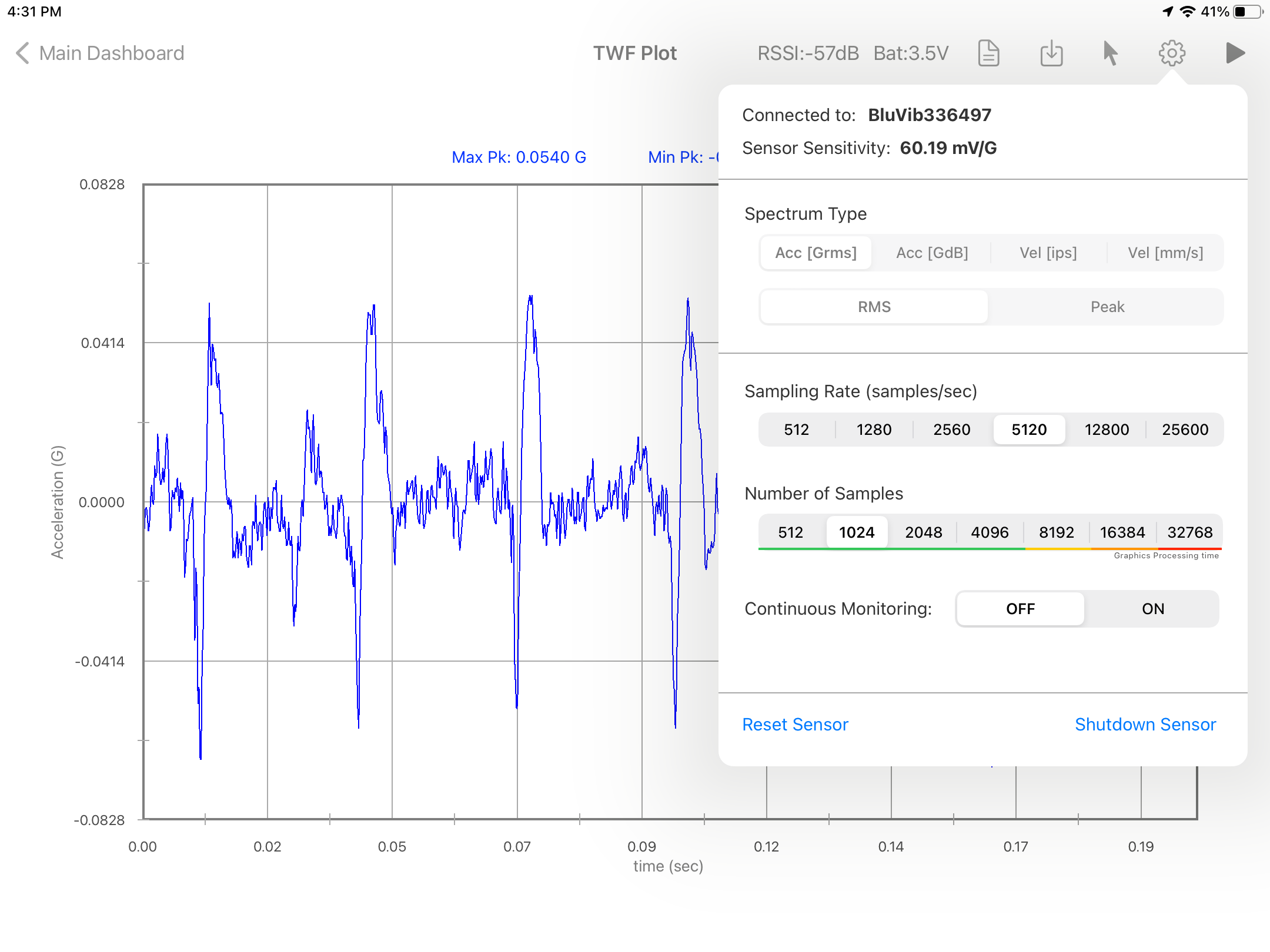
- After connecting/pairing the sensor, click on the start button to take a reading. To zoom the plot use both fingers to pinch in and out, to pan use one finger and swipe left or right. Other options, such as DC-Removal and Filters can be modified in the general Configuration view. See Configuration item 3 for more details
- The settings pop-up will allow the user to change the sampling rate and the number of samples. Here the user can select to turn ON the 'continuous mode' that will repeat data capturing and processing until stopped. Only a single-reading will be taken if the continuous mode is in the OFF position.
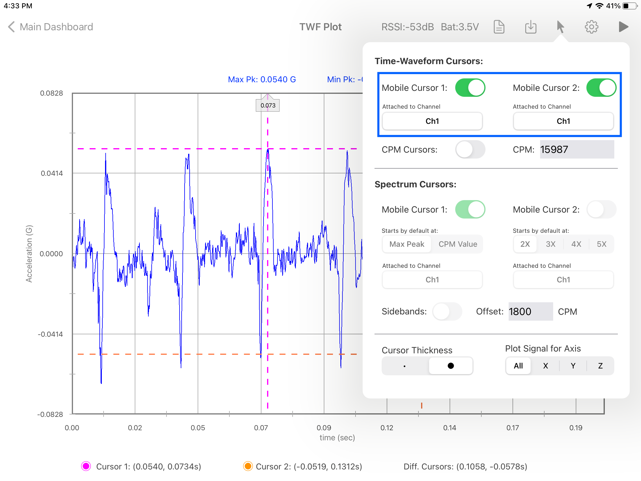
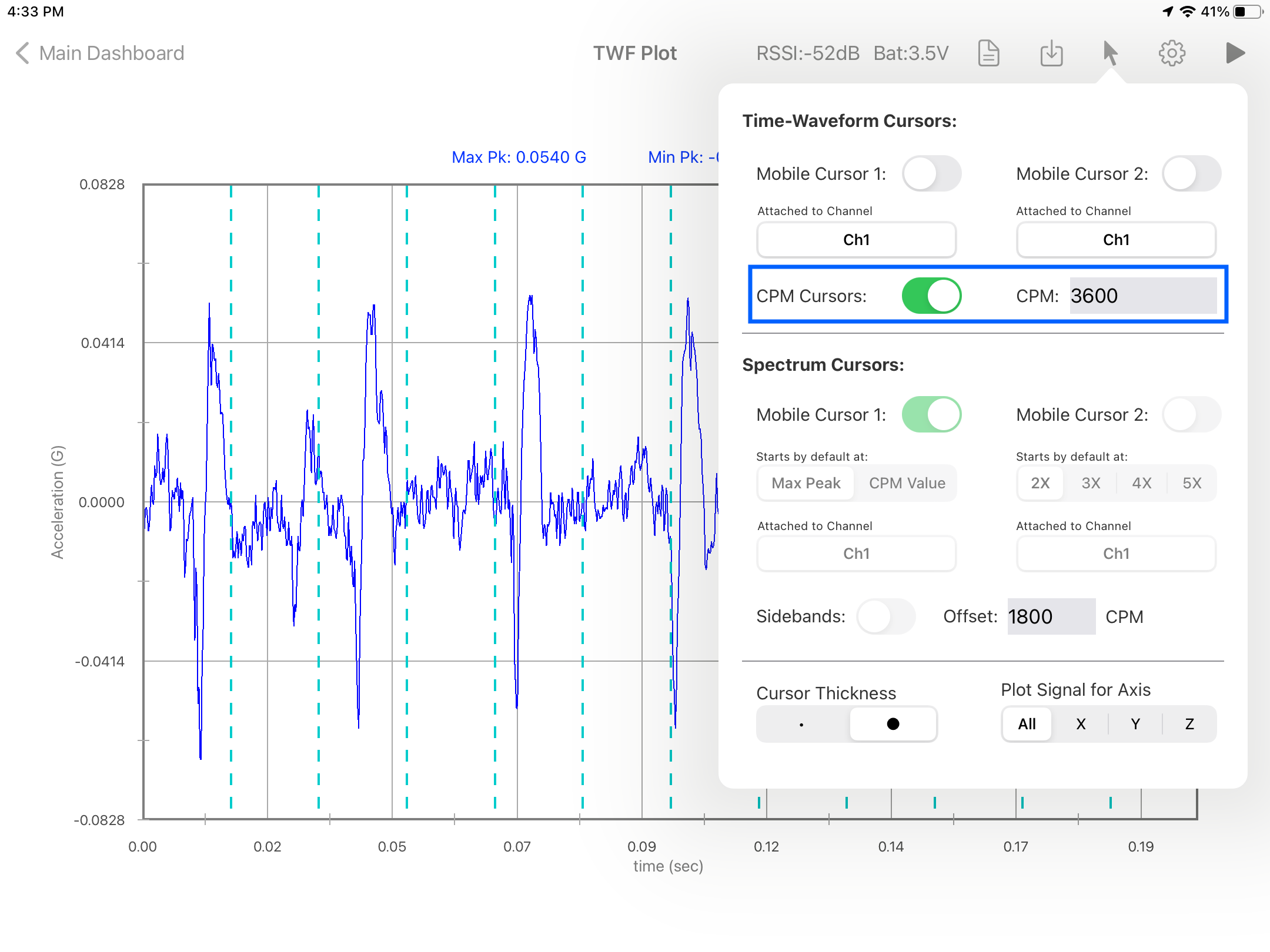
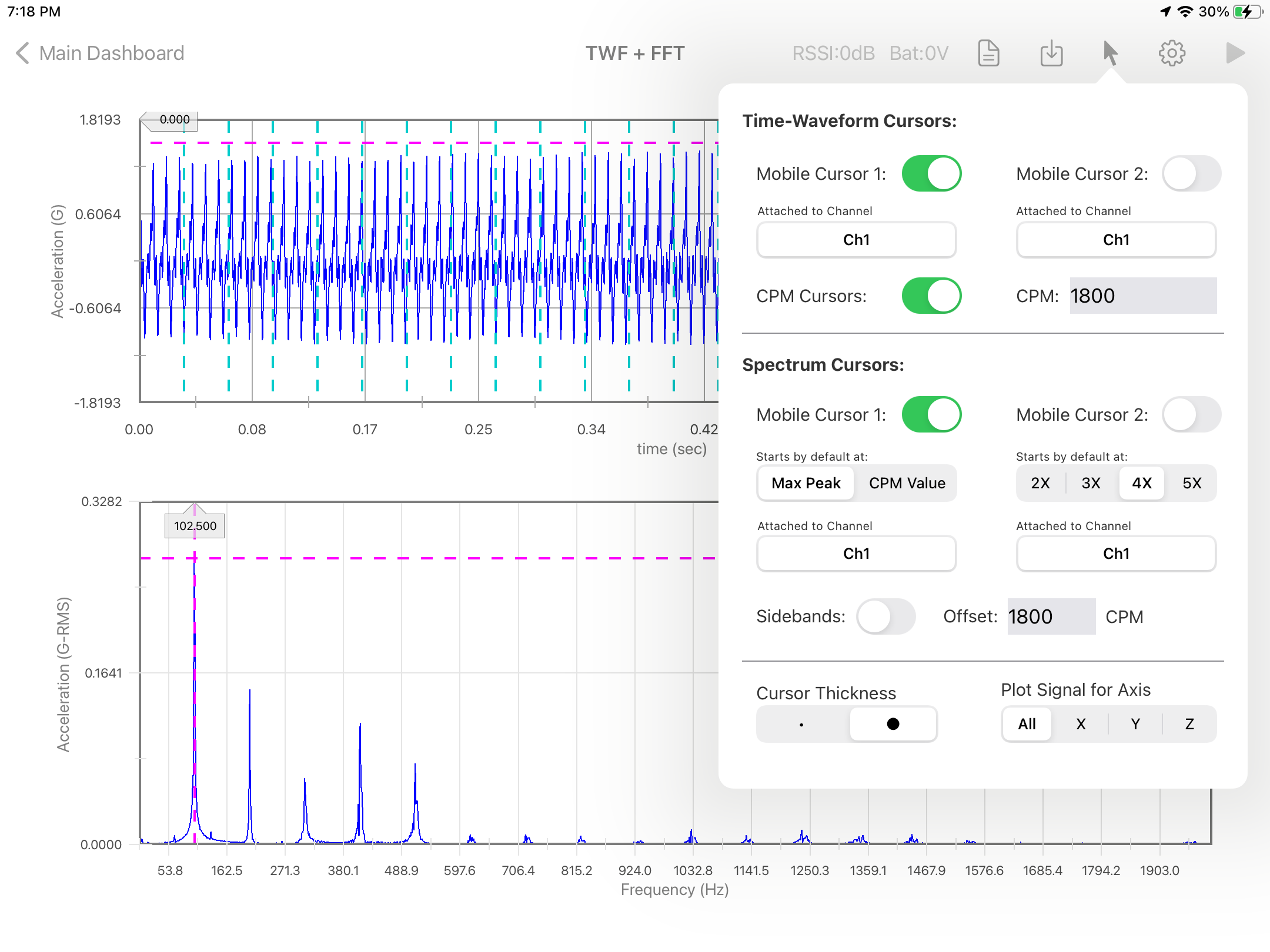
- The cursors pop-up will allow the user to add manual cursors or the CPM cycle cursor. The user can add a single manual cursor or a dual manual cursor by turning each switch on/off.
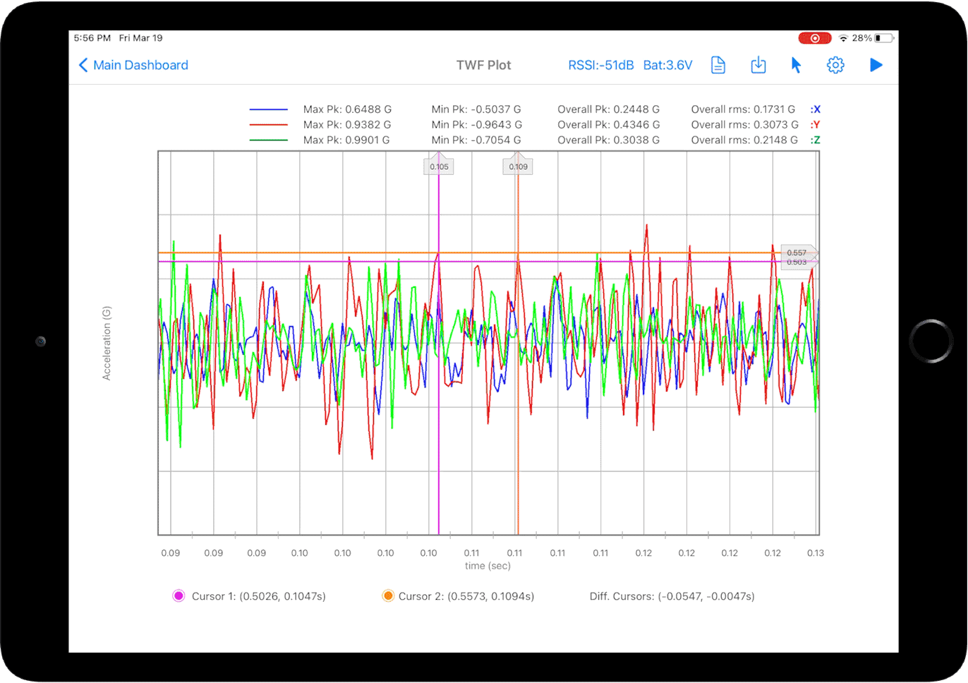
- For a 2 or 3 axis sensor, user can select the channel to attach the cursor (in the selector below the cursor switch), the case shown below is a triaxial signal and the cursor is attached to the Y-Axis (red color in the plot).
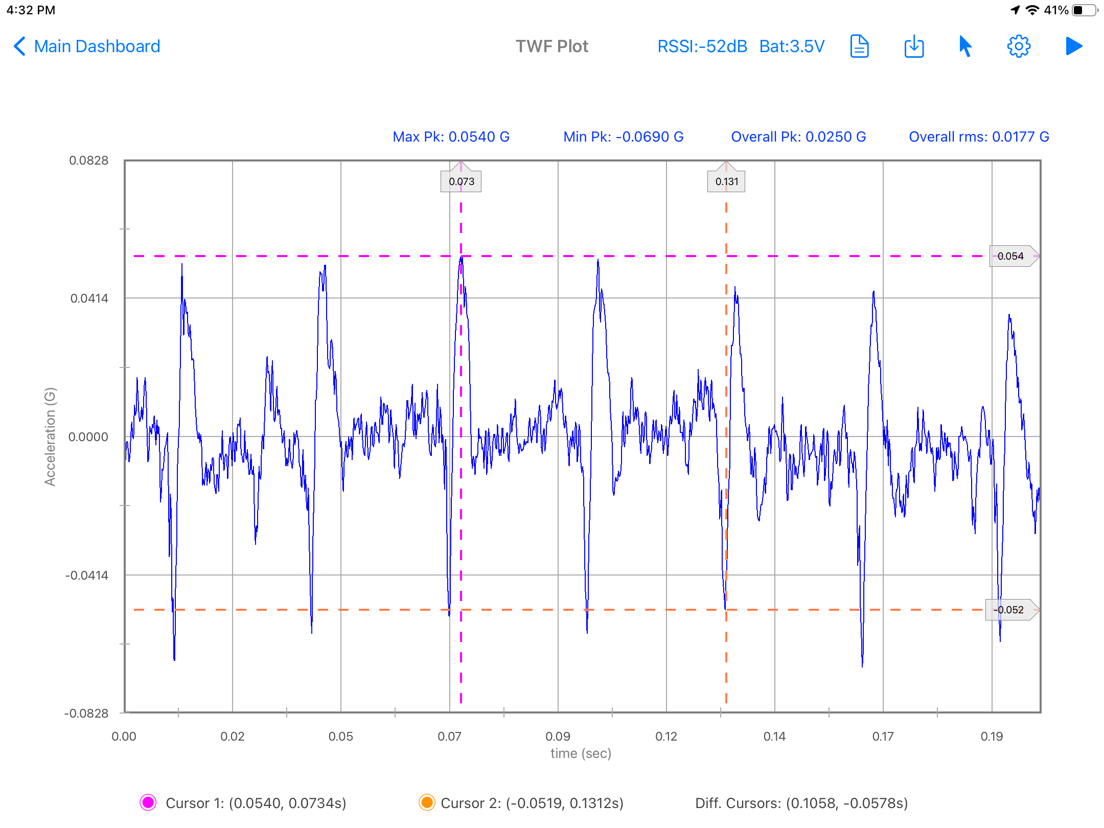
- User can drag the vertical (time) cursor 1 or 2 with the finger to any position, the horizontal (amplitude) cursor will follow the selected axis plot. The (Amplitude,Time) values for each cursor will appear in the bottom of the screen. The difference in amplitude and time will also be calculated and displayed on the bottom right corner of the screen.
- When the CPM cursor switch is ON, multiple cursors will appear to help define each vibration cycle in the time-waveform plot. Cycles are defined by the CPM value entered in the CPM field.
- The plot line and cursor thickness and style can be modified in the general "Configuration" screen from the main menu. More detail in the Configuration section items 1 and 2). All cursors can be toggled between a continuous or a segmented line.
- Data can be uploaded/downloaded from the cloud or saved/loaded locally by clicking on the save buton in the top bar menu, see more info in Saving data locally or in the cloud. A full pdf report can be generated, saved or sent by clicking on the report button, see more info in: Generating a pdf Report.
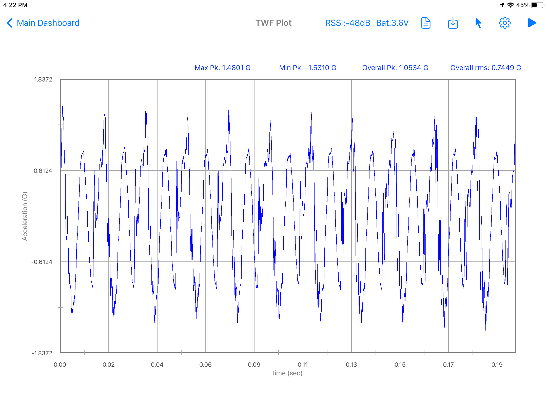
Note: For simplicity, a single-channel sensor will be used to explain all the functionalities
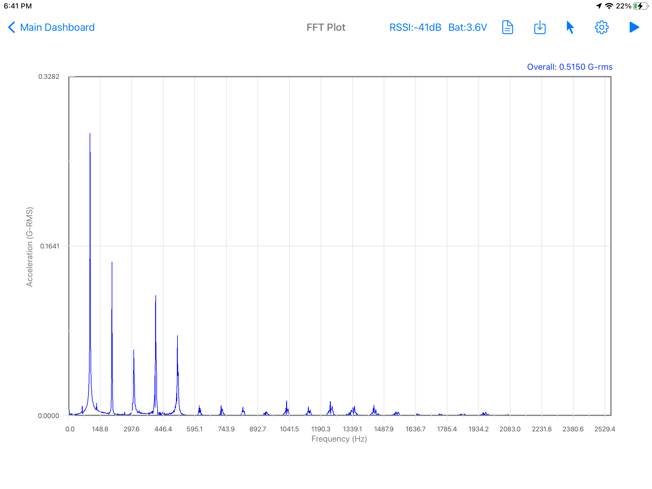
Spectrum
- After connecting/pairing the sensor, click on the start button to take a reading. To zoom the plot use both fingers to pinch in and out, to pan use one finger and swipe left or right. Other options, such as windowing, filtering and cut-off value can be modified in the general Configuration view. See Configuration item 4 for more details.
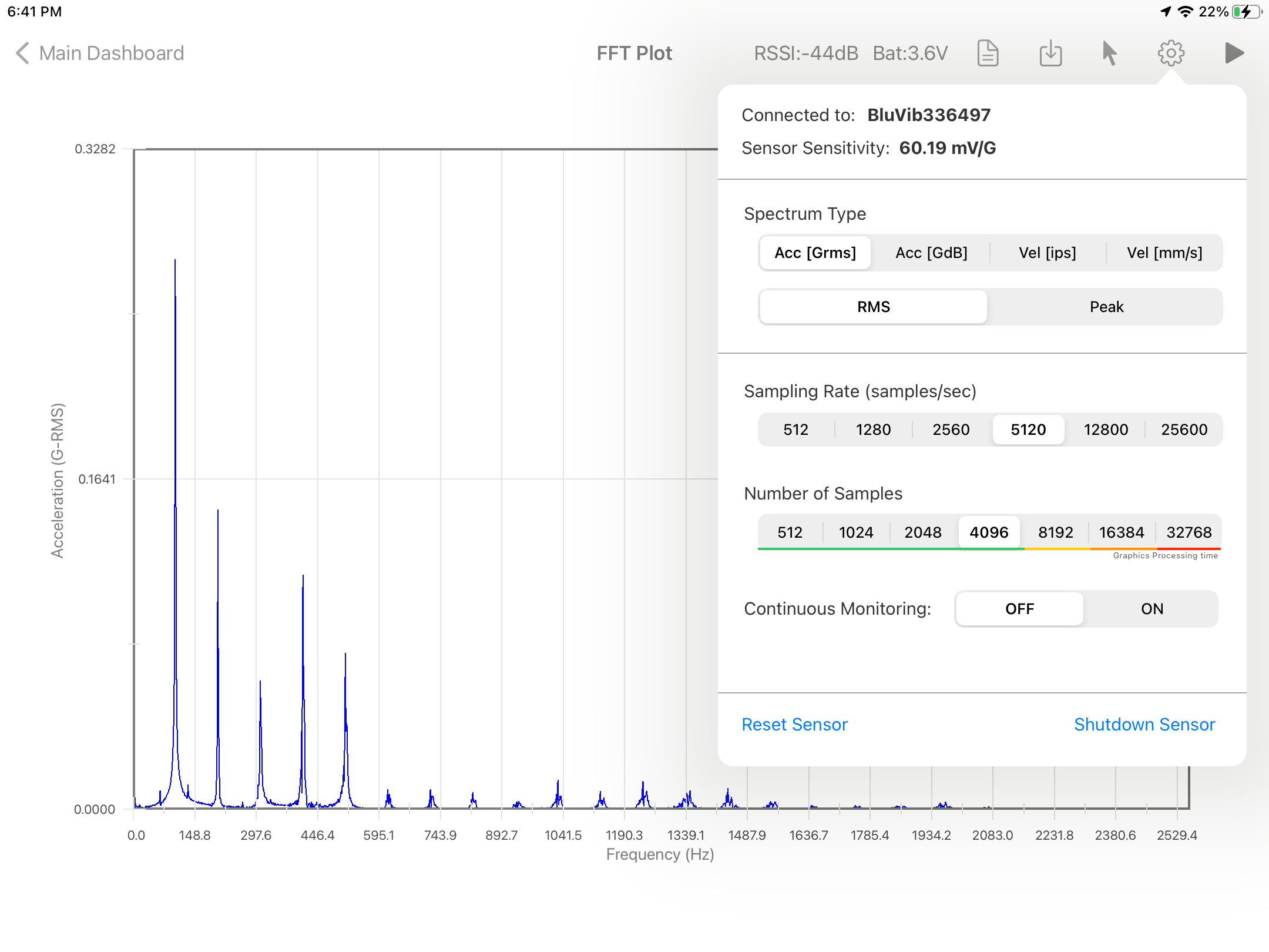
- The settings pop-up will allow the user to change the spectrum type to Acceleration in G's, Acceleration in dB and Velocity in ips or mm/s. The sampling rate and the number of samples can also be changed here, options will depend on the available sampling rate and number of samples of each sensor. Here the user can select to turn ON the 'continuous mode' that will repeat data capturing and processing until stopped. Only a single-reading will be taken if the continuous mode is in the OFF position.
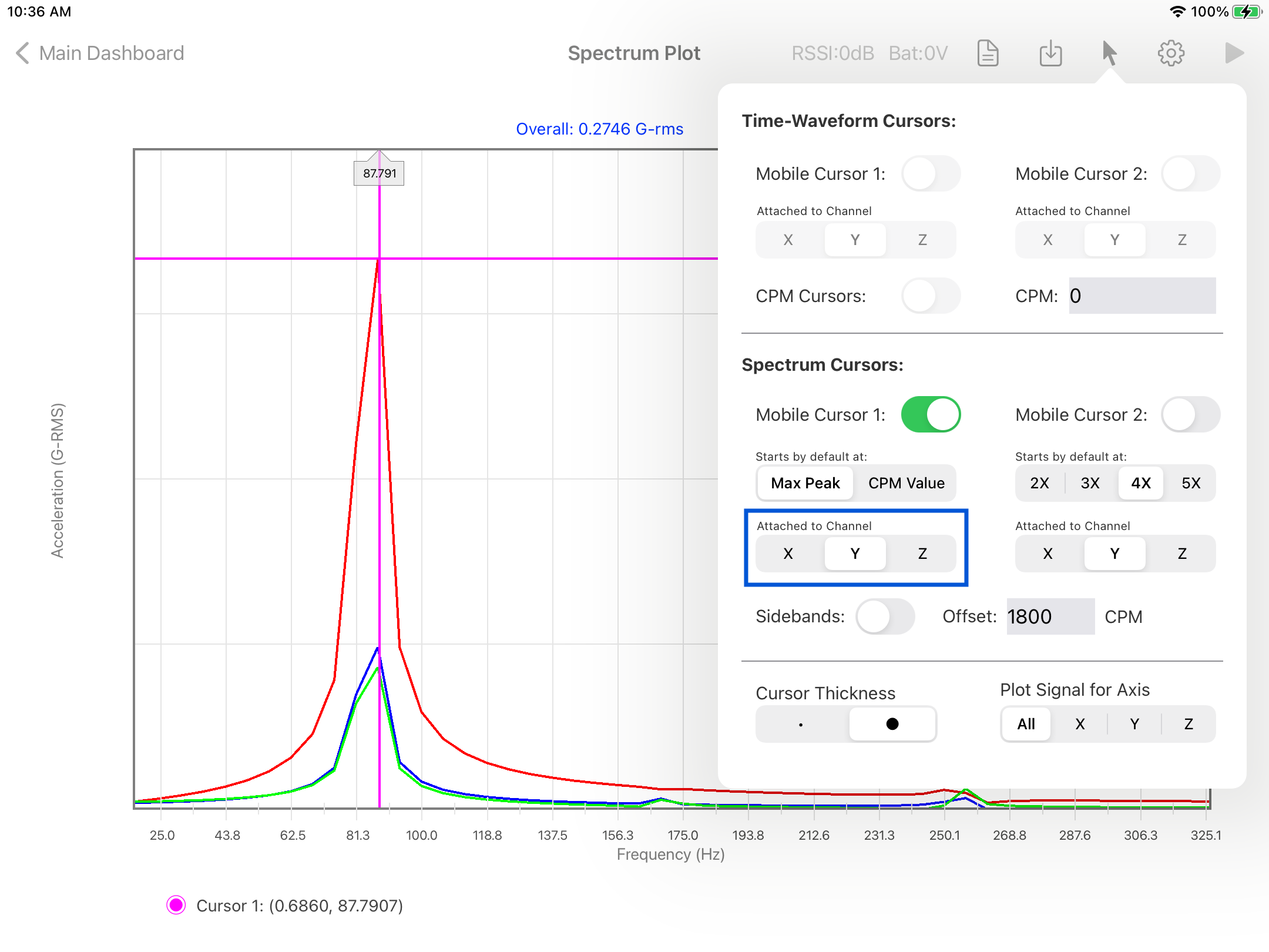
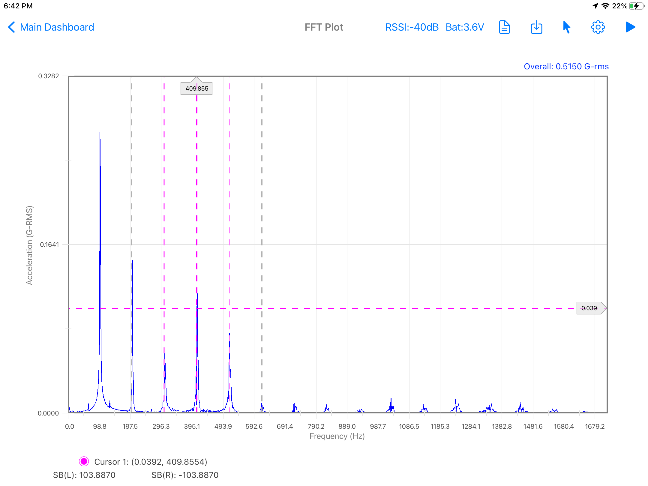
- In the cursors pop-up the user can add manual cursors, CPM cursor, Higher Peak cursor, harmonic cursors and sidebands cursors to the spectrum plot.
- For a 2 or 3 axis sensor, user can select the channel to attach the cursor (in the selector below the cursor switch), the case shown below is a triaxial signal and the cursor is attached to the Y-Axis (red color in the plot).
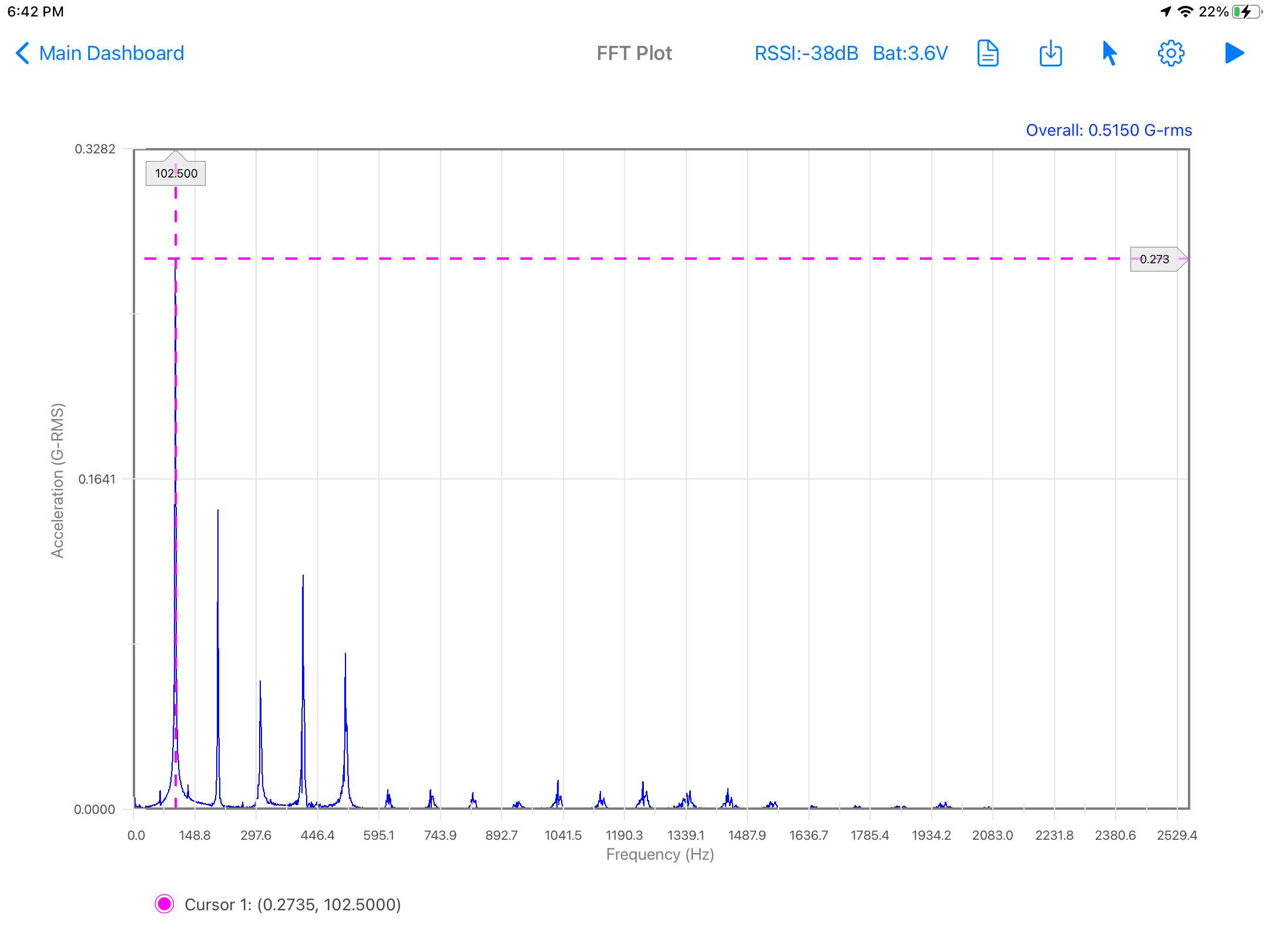
- By selecting the manual cursor 1, the user is given the option to automatically place it on the higher peak or on the entered CPM value. The vertical (frequency) cursor can be draged manually to the left or right, the horizontal (amplitude) cursor will follow the plot (on a triaxial plot, the user can select the axis to which the cursor is attached). The cursor position (amplitude, frequency) will be displayed on the bottom of the screen.
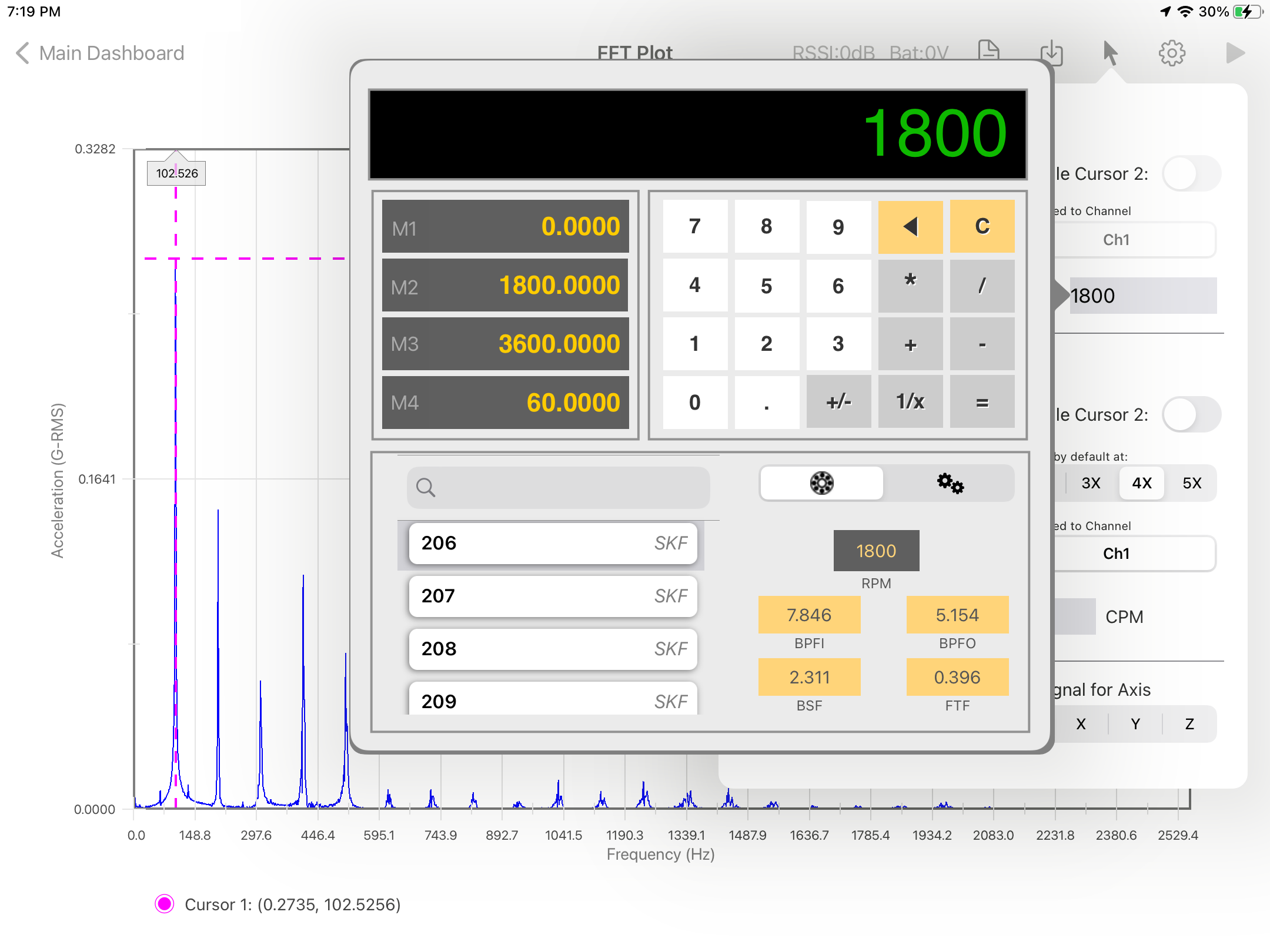
- The CPM value that defines the cursor position can be entered manually in the field using the frequency calculator. The calculator can also provide automatic calculation of bearing fault frequencies by selecting the bearing model from a list. Scroll to the desired bearing model and manufacturer or use the search bearing option, then enter the RPM in the calculator and it will calculate the fault frequency and place it in the cursor field.
- The frequency fault calculator can also calculate the Gear Mesh Frequency (GMF) by entering the number of teeth of the gear and its RPM.
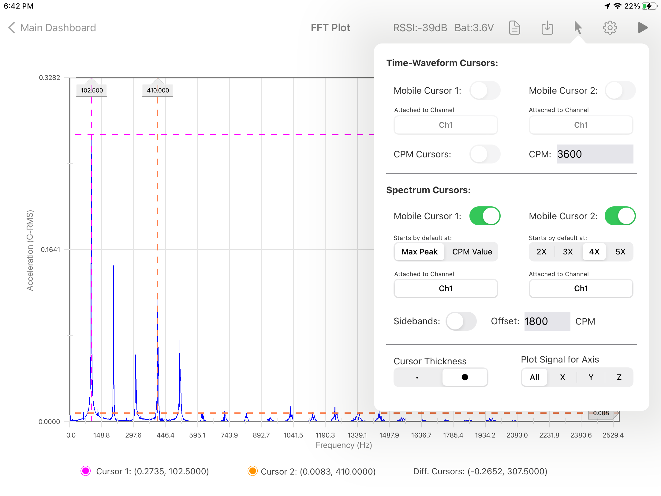
- The second manual cursor, can be used to calculate differences related to the cursor 1, or can be used to add harmonic cursors by selecting 2X, 3X, 4x or 5X. This will place the second cursor in the desired position related to the first. The position values (amplitude, frequency) of the second cursor will be displayed below the spectrum, together with the differences values. This cursor can be also dragged to any other position on the spectrum.
- The sidebands cursor, when selected, will appear around the cursor 1 with an initial separation as specified in the 'Offset' field'.
- By dragging the cursor 1, all the sidebands will move in accordance, maintaining the offset. The first family of sidebands can also be dragged to the left or right, increasign the offset of the first family and the offset of the second family in the right proportions.
- Data can be uploaded/downloaded from the cloud or saved/loaded locally by clicking on the save buton in the top bar menu, see more info in Saving data locally or in the cloud.
- A full pdf report can be generated, saved or sent by clicking on the report button, see more info in: Generating a pdf Report.
Note: For simplicity, a single-channel sensor will be used to explain all the functionalities


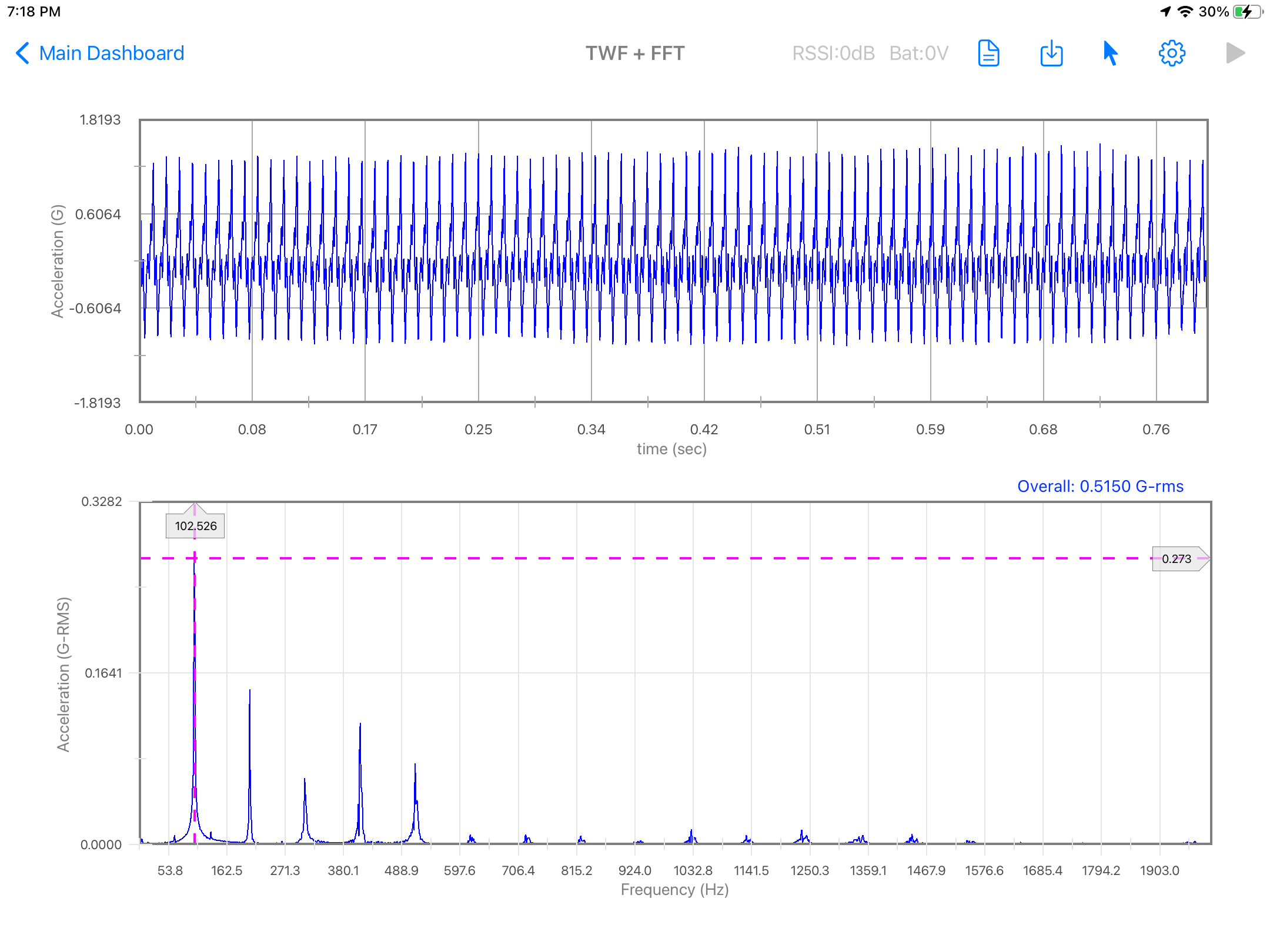
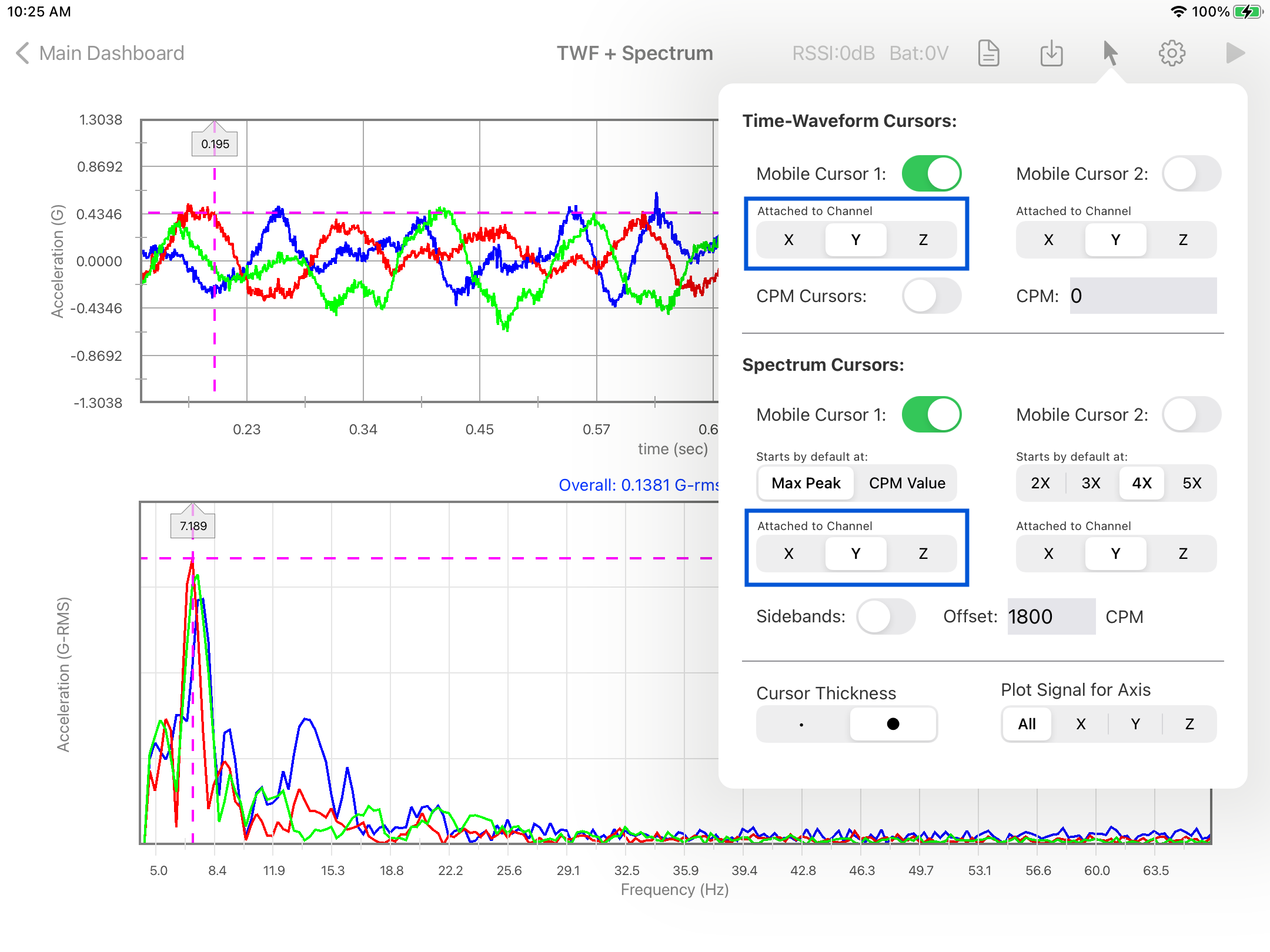
TWF & Spectrum
- After connecting/pairing the sensor, click on the start button to take a reading. To zoom the plot use both fingers to pinch in and out, to pan use one finger and swipe left or right. Other options, such as DC-Removal, filters, windowing and cut-off value can be modified in the general Configuration view. See Configuration item 3 and 4 for more details
- The settings pop-up will allow the user to change the spectrum type to Acceleration in G's, Acceleration in dB and Velocity in ips or mm/s. The sampling rate and the number of samples can also be changed here, options will depend on the available sampling rate and number of samples of each sensor. Here the user can select to turn ON the 'continuous mode' that will repeat data capturing and processing until stoped. Only a single-reading will be taken if the continuous mode is in the OFF position.
- In the cursors pop-up the user can add manual cursor and CPM cursors to the Time-Waveform and manual cursors, CPM cursor, Higher Peak cursor, harmonic cursors and sidebands cursors to the spectrum plot. For more details refer to the Time-Waveform or to the Spectrum sections for details of each cursor operation.
- In case of a 2 or 3 axis sensor, user can select the channel to attach the cursor in the selector for each cursor, in the sample below both (TWF & FFT) cursors are attached to the Y-Axis (shown in red in the plot).
- Data can be uploaded/downloded from the cloud or saved/loaded locally by clicking on the save buton in the top bar menu, see more info in Saving data locally or in the cloud.
- A full pdf report can be generated, saved or sent by clicking on the report button, see more info in: Generating a pdf Report.
Note: For simplicity, a single-channel sensor will be used to explain all the functionalities
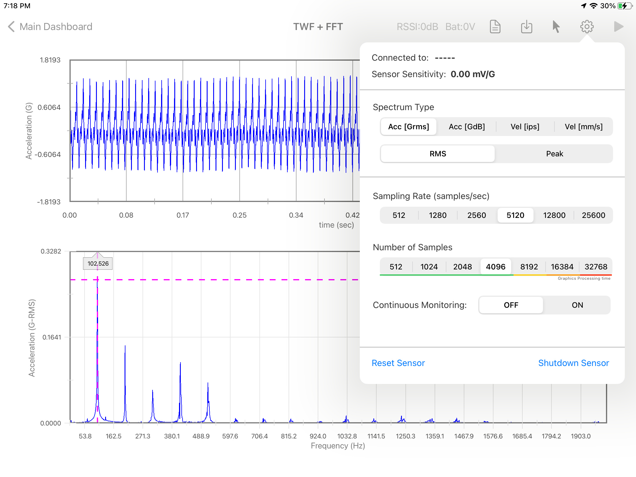
Configuration
- From the Main menu, click the top left menu button to open the left drawer with more options. Select 'Configuration' from the left menu
- Select the Plot Thickness, Cursor Thickness and/or Cursor Line Type from the Plot Settings selectors.
- The Signal Settings will affect the raw data directly. The DC-Removal is ON by default by can be turned OFF here. Also a general Low-Pass or High_pass filter can be applied to the signal.
- The FFT Settings will be set as defaults for all readings. Here the user can change the spectrum frequency units to Hz, CPM or Orders. A Cut-Off value can be added to remove low frequency values. Also windowing can be selected for the spectrum, the available options are: None, Hanning, Hamming, Blackman, Nutall and Flat-Top. The spectrum type and RMS/Pk values can be set as defaults here, but can also be changed in the settings pop-up of the spectrum.
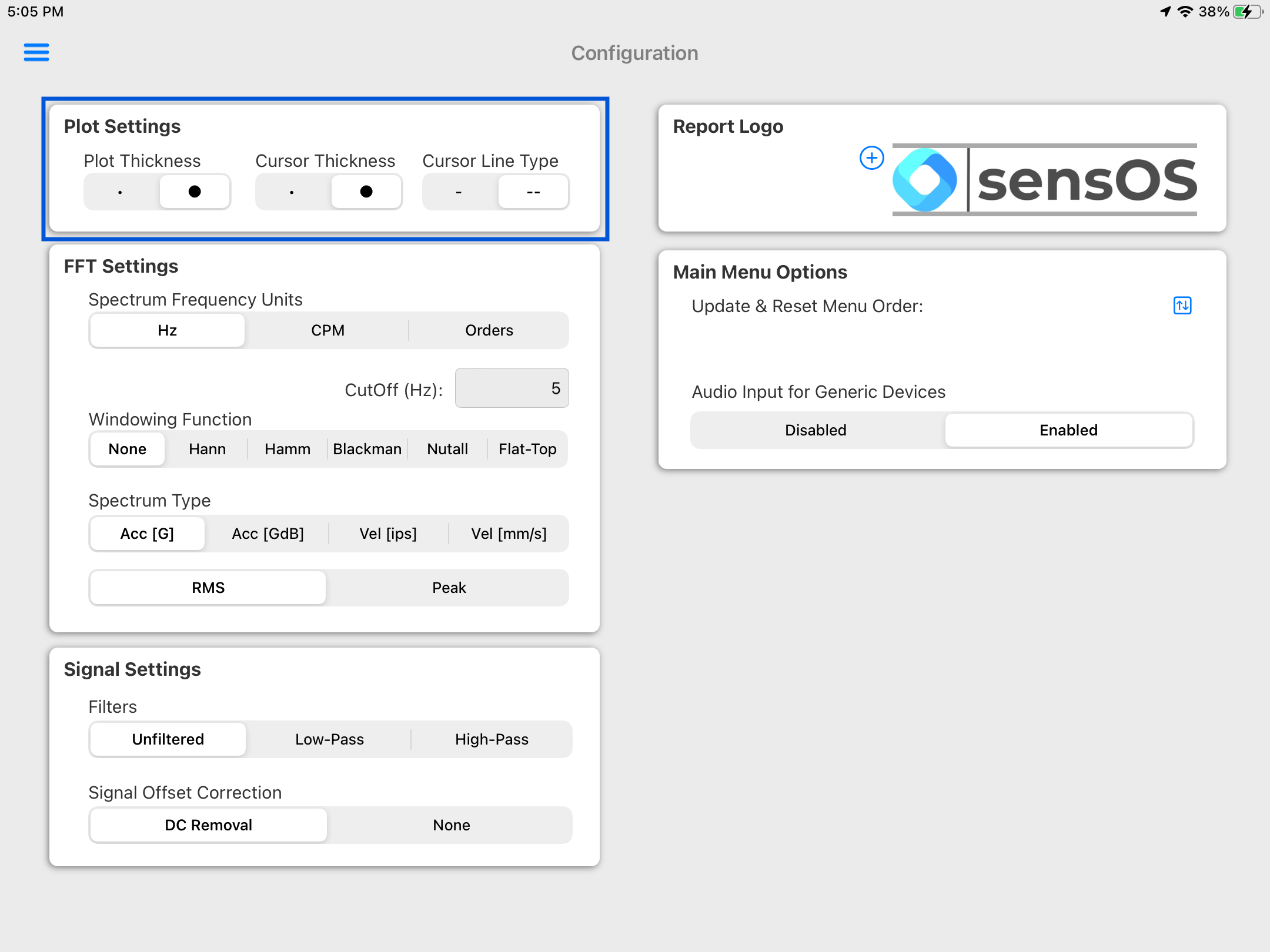
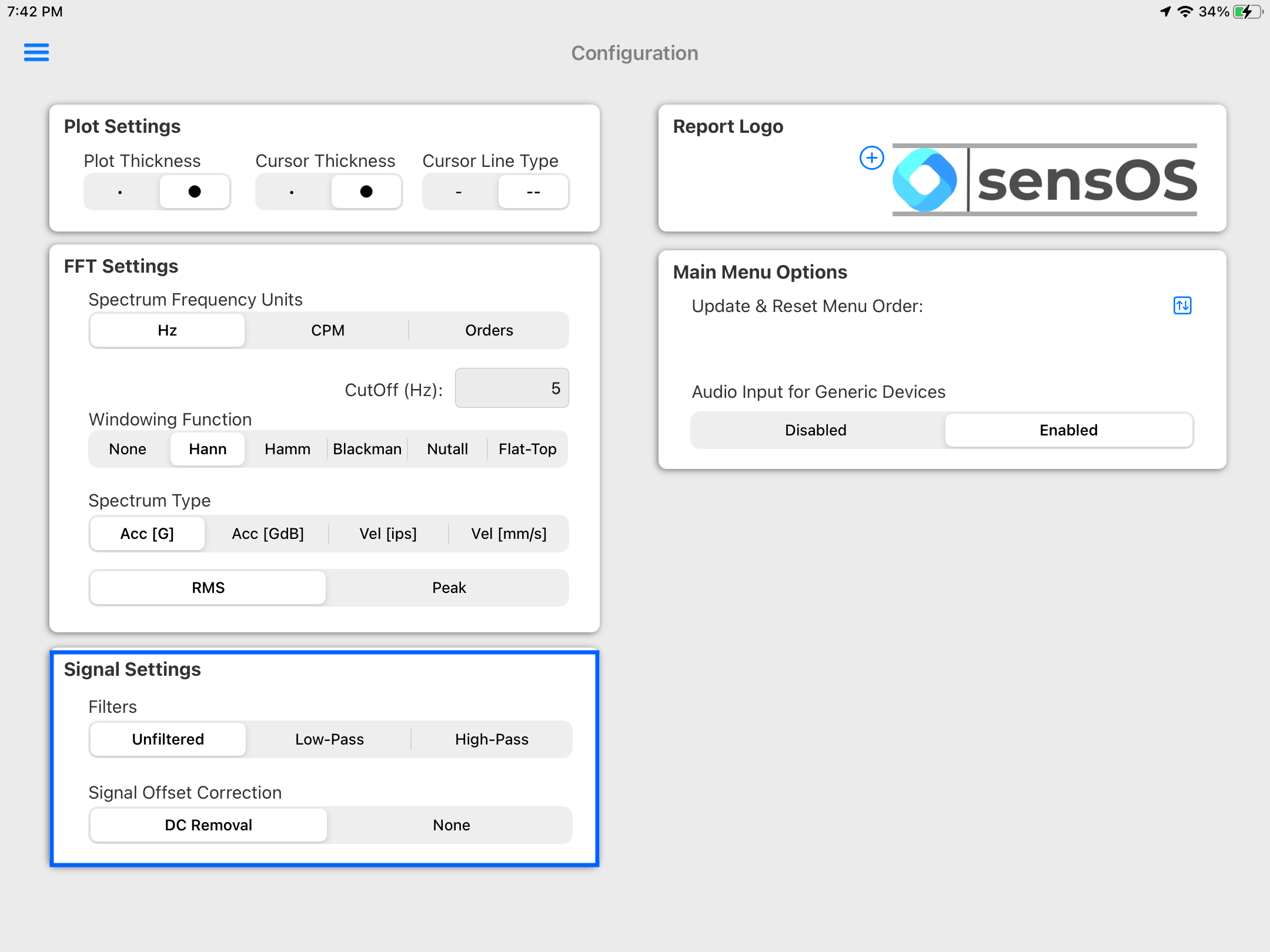
Note: This selection will affect all reading's raw data for all modules

Report
- Clicking on the Report button will open a new view with the pdf report.
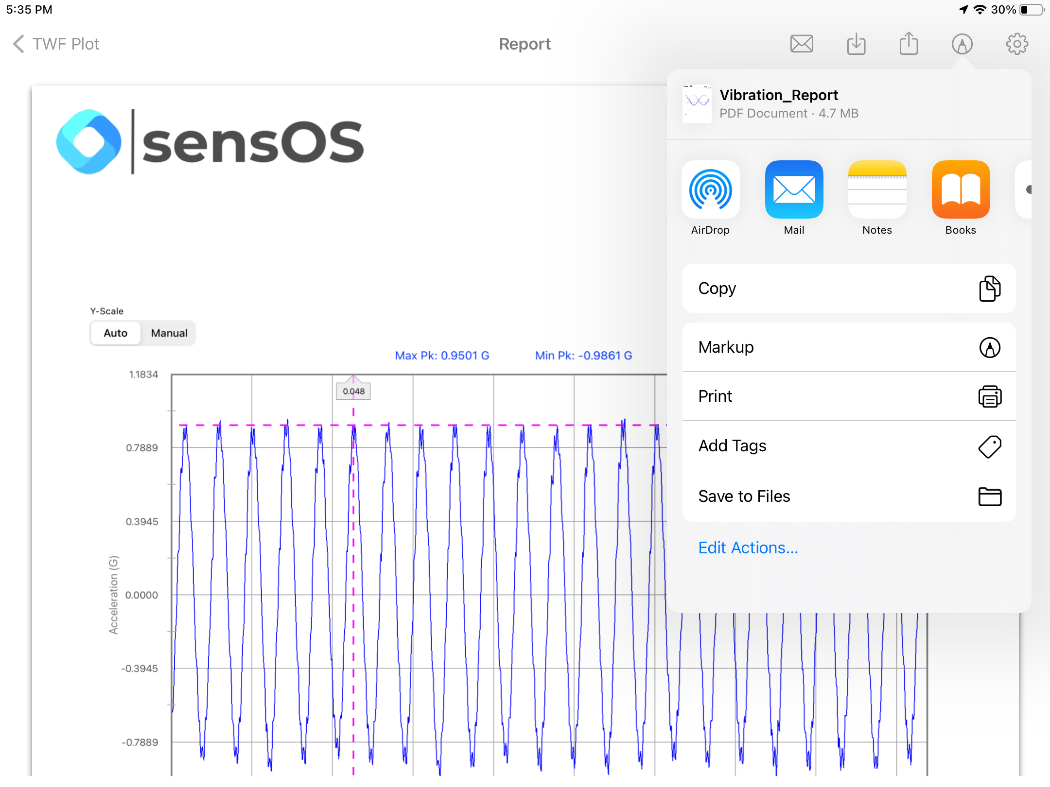
- The report view contains several options in the top bar menu: 1:Send by Email, 2:Save pdf locally, 3:Upload Report to the Cloud bucket, 4:Markup and 5:Report Configuration
- The markup tool allows the user to copy the report to the clipboard, send it by Airdrop or any other messaging app, email it, print it or saved it to Files. The markup tool will open the standard tool to paint on the pdf report.
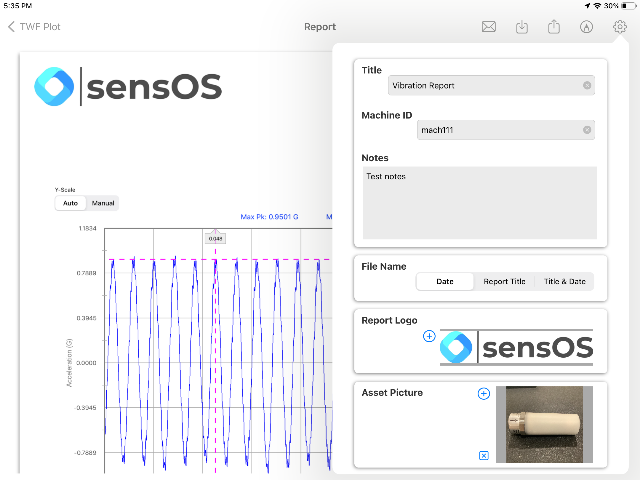
- The Report Configuration pop-up allows the user to enter the Report Title, Machine ID and Notes to be added to the report. Here the user can also select a logo for the report and include a picture of the asset that will be added in a new page in the report. The report file name be default is the actual dat and time, but the user can change it to the title name of the report or to both, the title name and date.


Files & Data
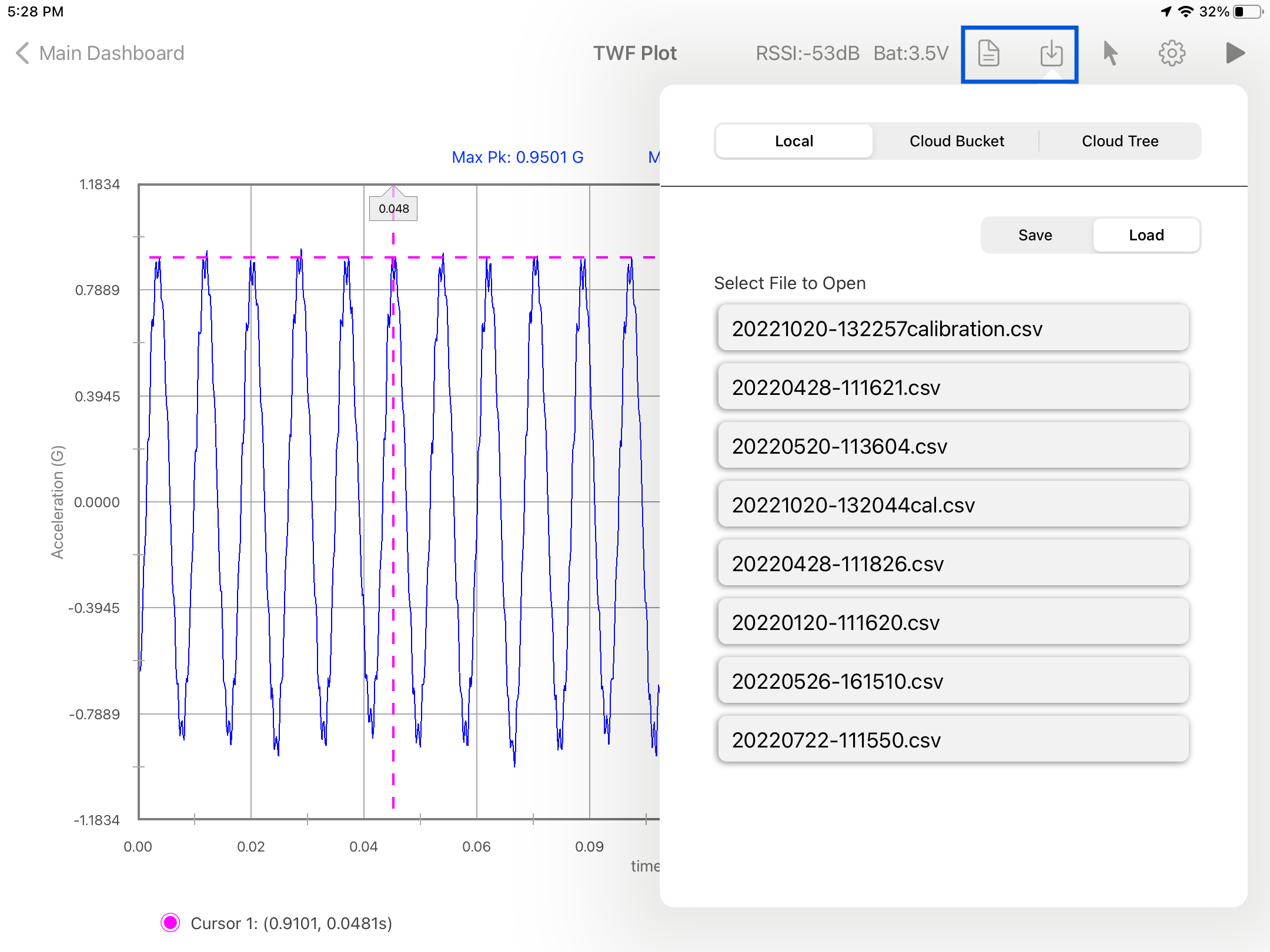
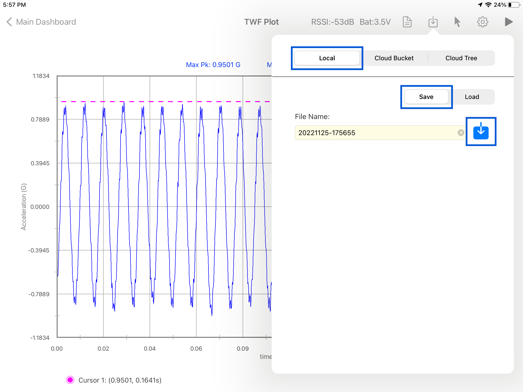
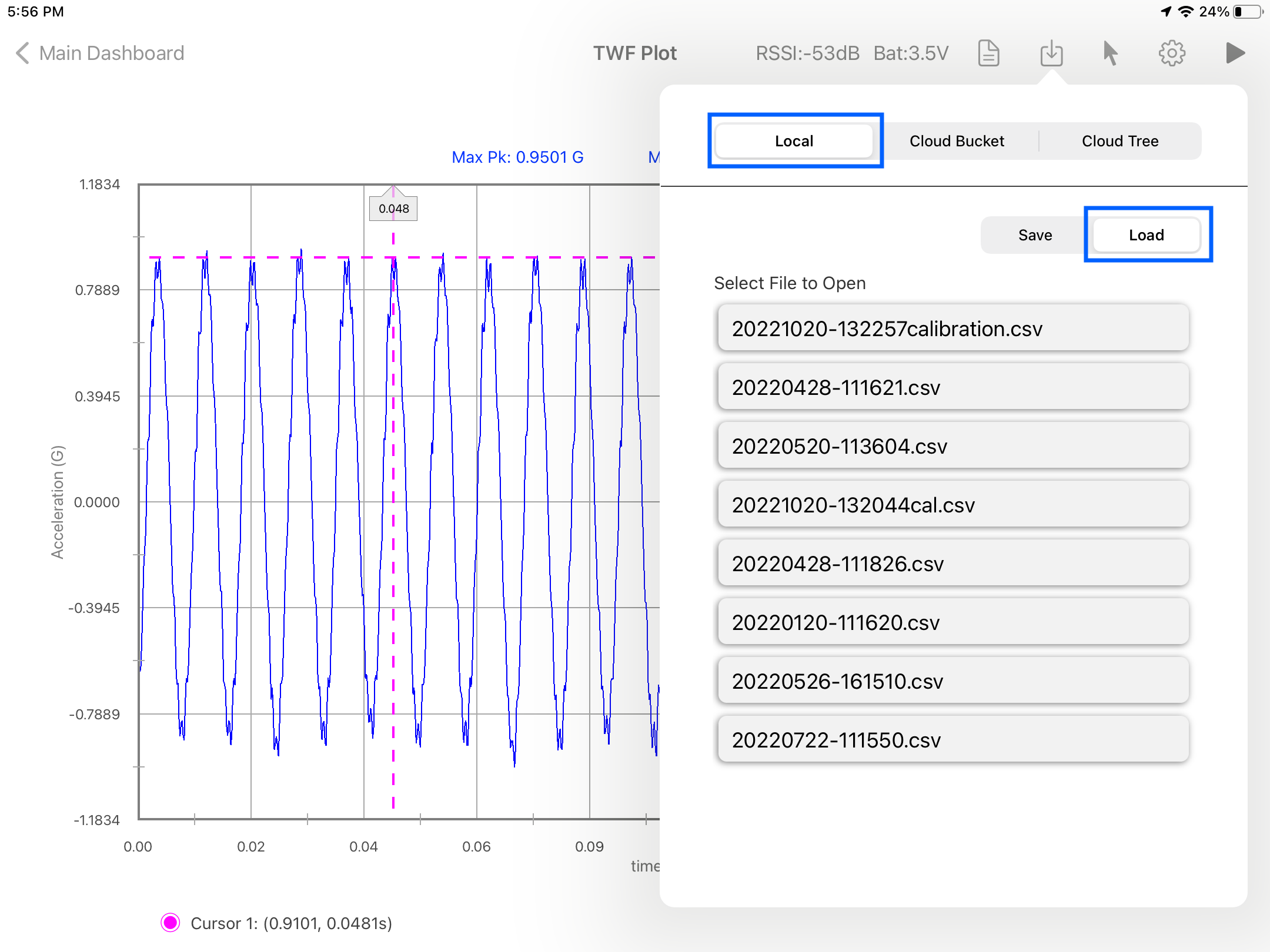
- By selecting the Files & Data button in the top bar, the user can save/load the vibration data locally, in the cloud bucket or in the cloud hierarchy tree.
- To save data locally, select the 'Local' option in the first selector and then select 'Save' in the selector below. By default the name of the file will be the timestamp, but the user can customize it here and click on the blue save button on the right.
- To load data locally, select the 'Local' option in the first selector and then select 'Load' in the selector below. A list of all available local files will appear, tap on the desired file and it will load and process in the actual plot.
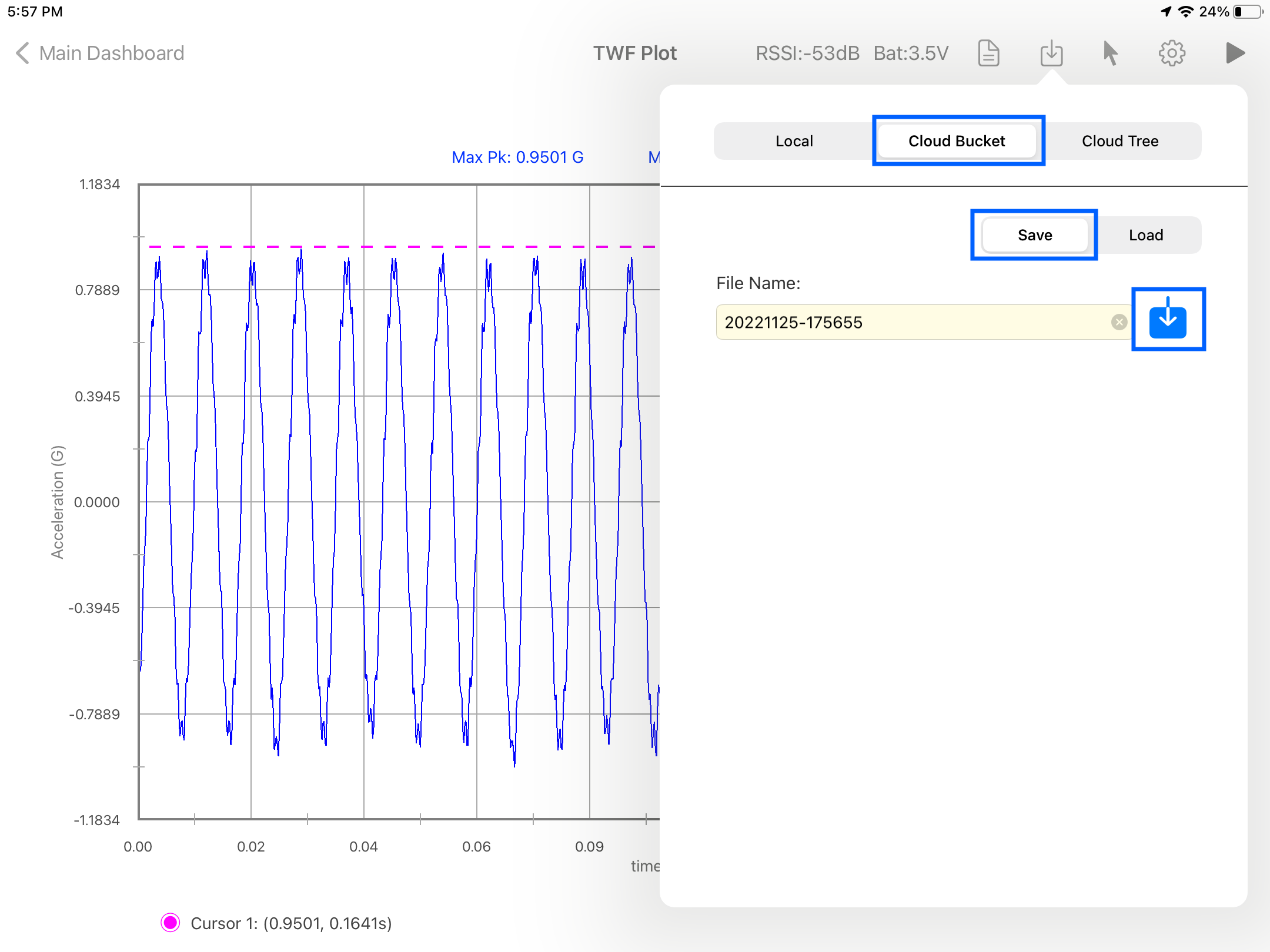
- To save data on the user's cloud bucket, select the 'Cloud Bucket' option in the first selector and then select 'Save' in the selector below. By default the name of the file will be the timestamp, but the user can customize it here and click on the blue save button on the right, this will upload the data file to the user's cloud bucket.
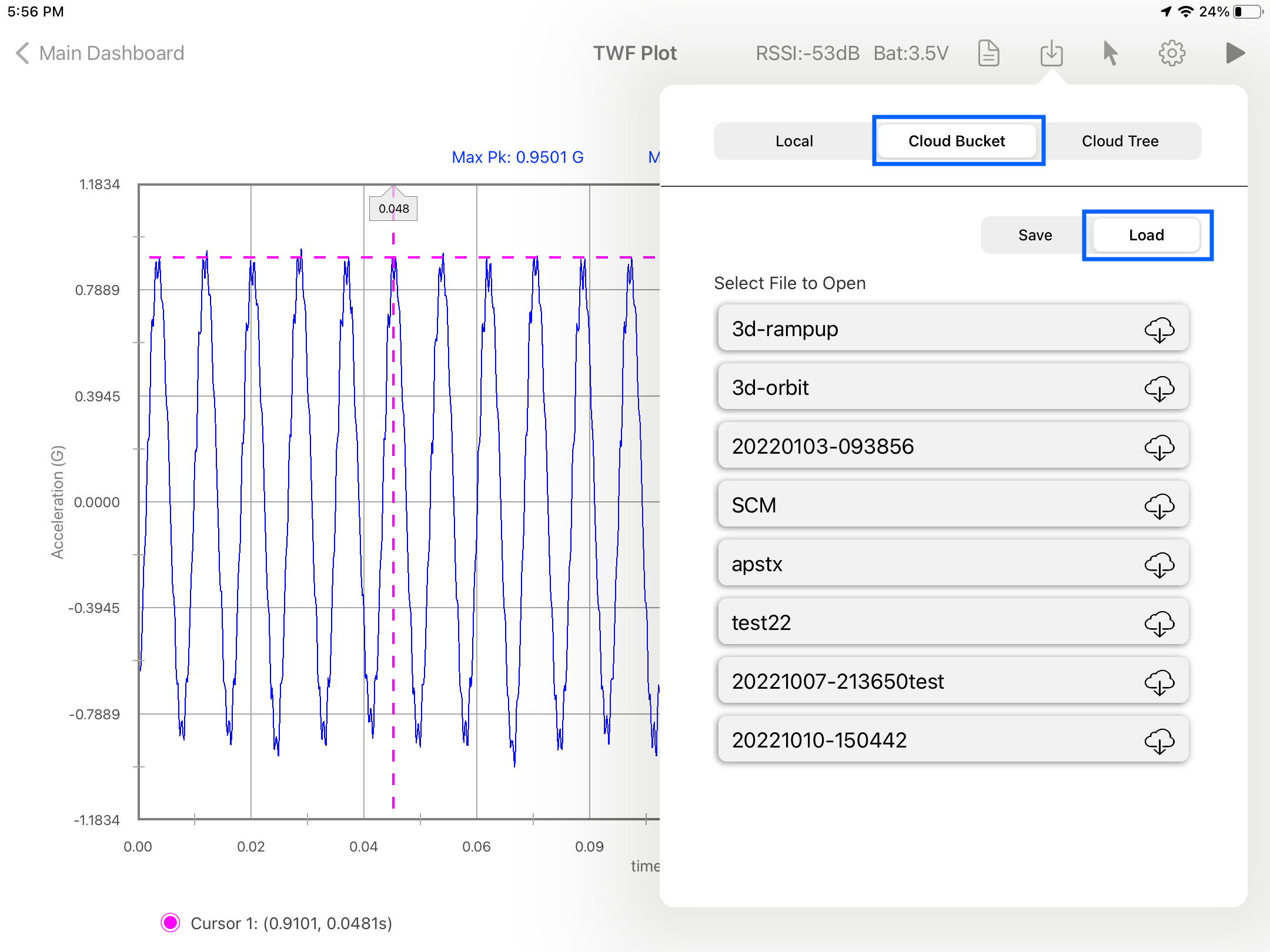
- To load data from the user's cloud bucket, select the 'Cloud Bucket' option in the first selector and then select 'Load' in the selector below. A list of all available local files will appear, tap on the desired file and it will load and process in the actual plot.
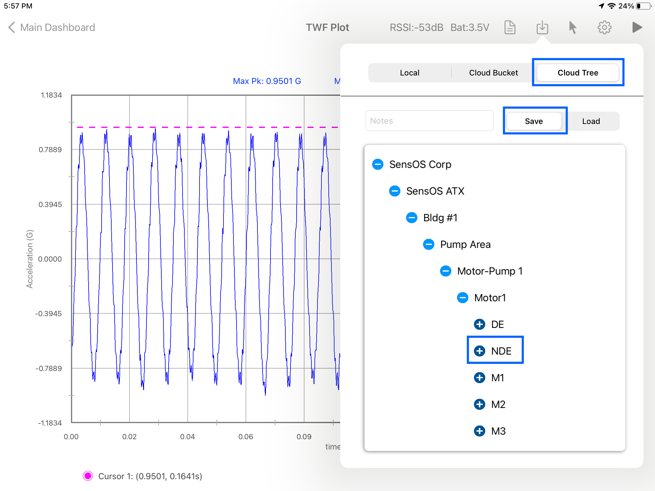
- To save data on the user's hierarchy tree, select the 'Cloud Tree' option in the first selector and then select 'Save' in the selector below. The user's hierarchy tree will appear, navigate to the point to save the data by clicking on each location, machine, component, and point.
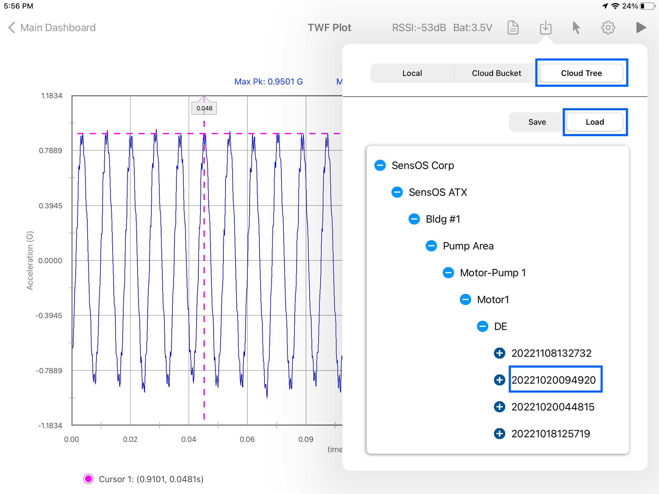
- To load data from the user's hierarchy tree, select the 'Cloud Tree' option in the first selector and then select 'Load' in the selector below. The user's hierarchy tree will appear, navigate to the desired reading (timestamp) by clicking on the desired locations, machine, component and point.

Changelog
See what's new added, changed, fixed, improved or updated in the latest versions.
Version 1.49 b.126 (21 Nov, 2022)
- Optimized Optimized for iPadOS 16
Version 1.33 b.103 (24 Feb, 2022)
- Fixed Bug Fixed
Version 1.01 b.51 (04 Mar, 2021)
Initial Release