Documentation
4434 Single-Plane Balancing
MS-4434: Rotor Balancing Studio iPadOS® version
- Version: 1.23 (b.59)
- Author: D. Bukowitz
- Created: 05 Oct, 2021
- Updated: 30 Apr, 2025
If you have any questions that are beyond the scope of this document, Please feel free to email via info@sens-os.com
Description
The Single-Plane Balancing Method included in the MS-4434 App was specially designed to balance rigid rotors over a wide range of speeds. The entire process is carried out by guiding the user step by step through a series of screens that are better explained throughout this document.
The following diagram describes the architecture and flow diagram of the Single-Plane Balance (click the image to zoom).

Compatibility
This module is compatible with the following sensors:
- EI-WiSER™3X (4-Channel Wireless)
- EI-WiSER™1X (2-Channel Wireless)
- Digital ICP Signal Conditiones (2-Channel Wired)
- EI-Wiser™ (2-Channel Wireless)
- Generic wired DAU (2-Channel Wired)
- TPI-9043 (3-Channel Wireless)
Main Menu
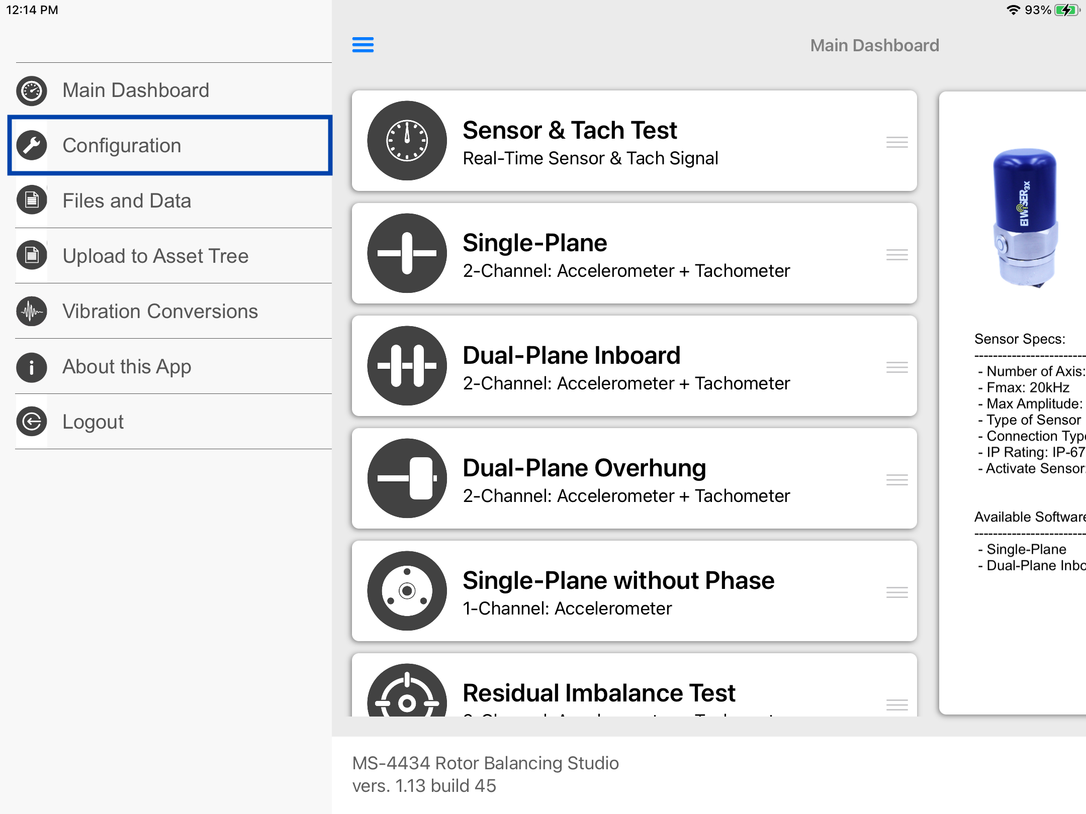
- Tap on the Sensor name button to open the list of available sensors, and select the sensor from the list
- Scroll the list of functionalities and select Single-Plane

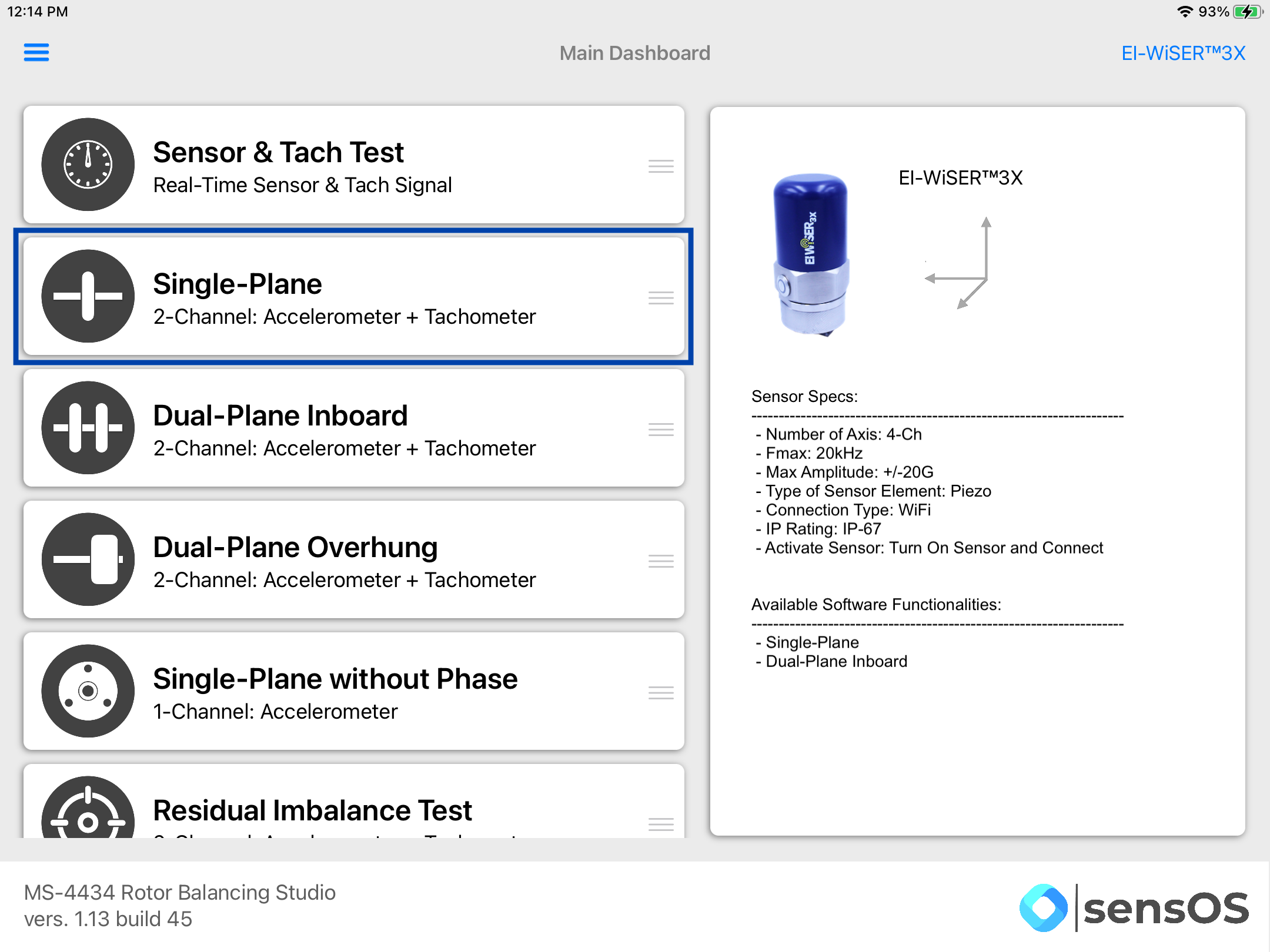
Note: The user can change the order of the functionalities in the list by dragging it from the right button on each cell
Single-Plane Balancing
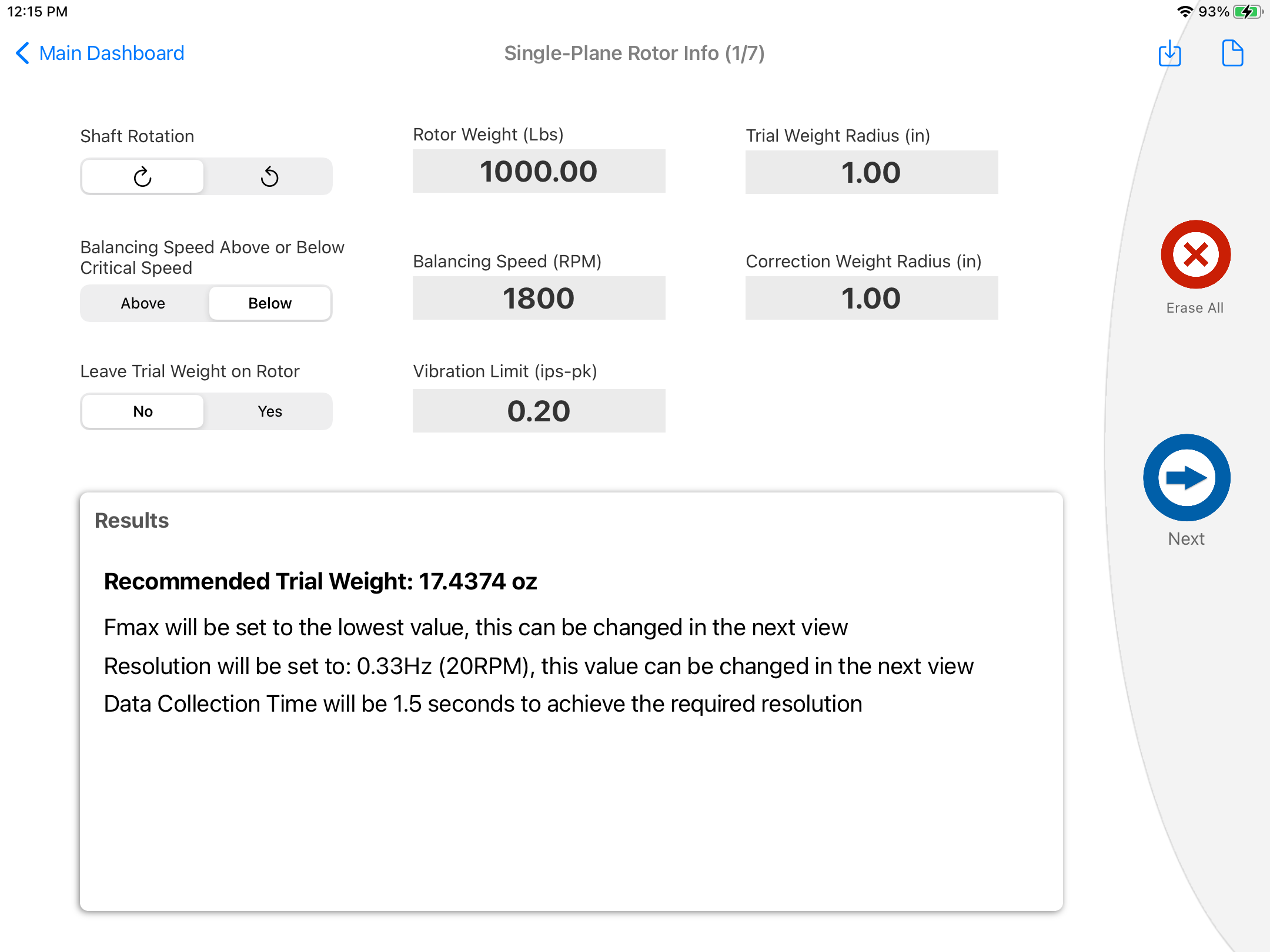
- In the first view (1 of 7) the user can define the basic parameters of the rotor and balancing process. Once the user defines these values and conditions, the system will set the best combination of sampling settings for the selected sensor and will provide a recommended trial weight. These sampling settings and the trial weight can be changed later on each screen while balancing. Click on the "Erase All" button to clear all fields. Previously saved data for this machine can be downloaded from the MS-Cloud Platform, see more details in Files & Data. Pressing the "Report" button will take the user directly to the report of the actual balancing job. To continue balancing press the "Next" button.
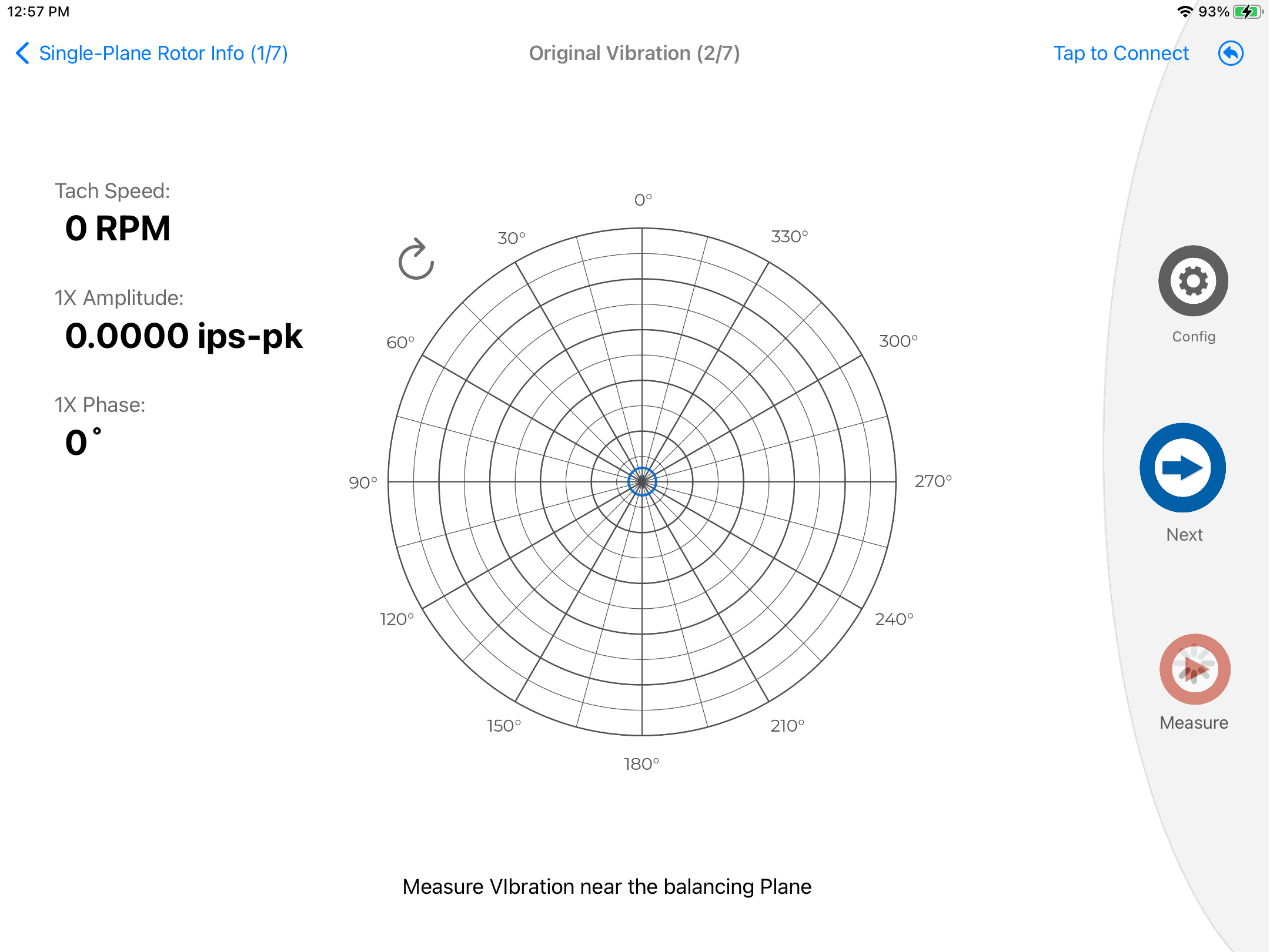
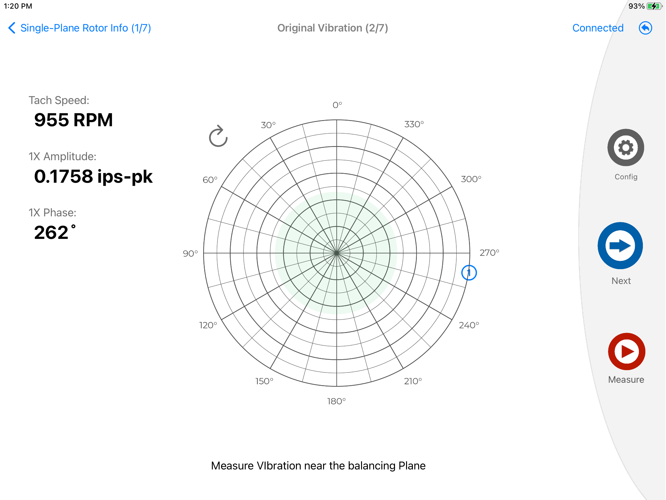
- The next view (2 of 7) will record the Original Vibration vector of the rotor. Turn on the sensor, mount it together with the tach on the machine and click on the "Tap to Connect" button in the top bar menu.
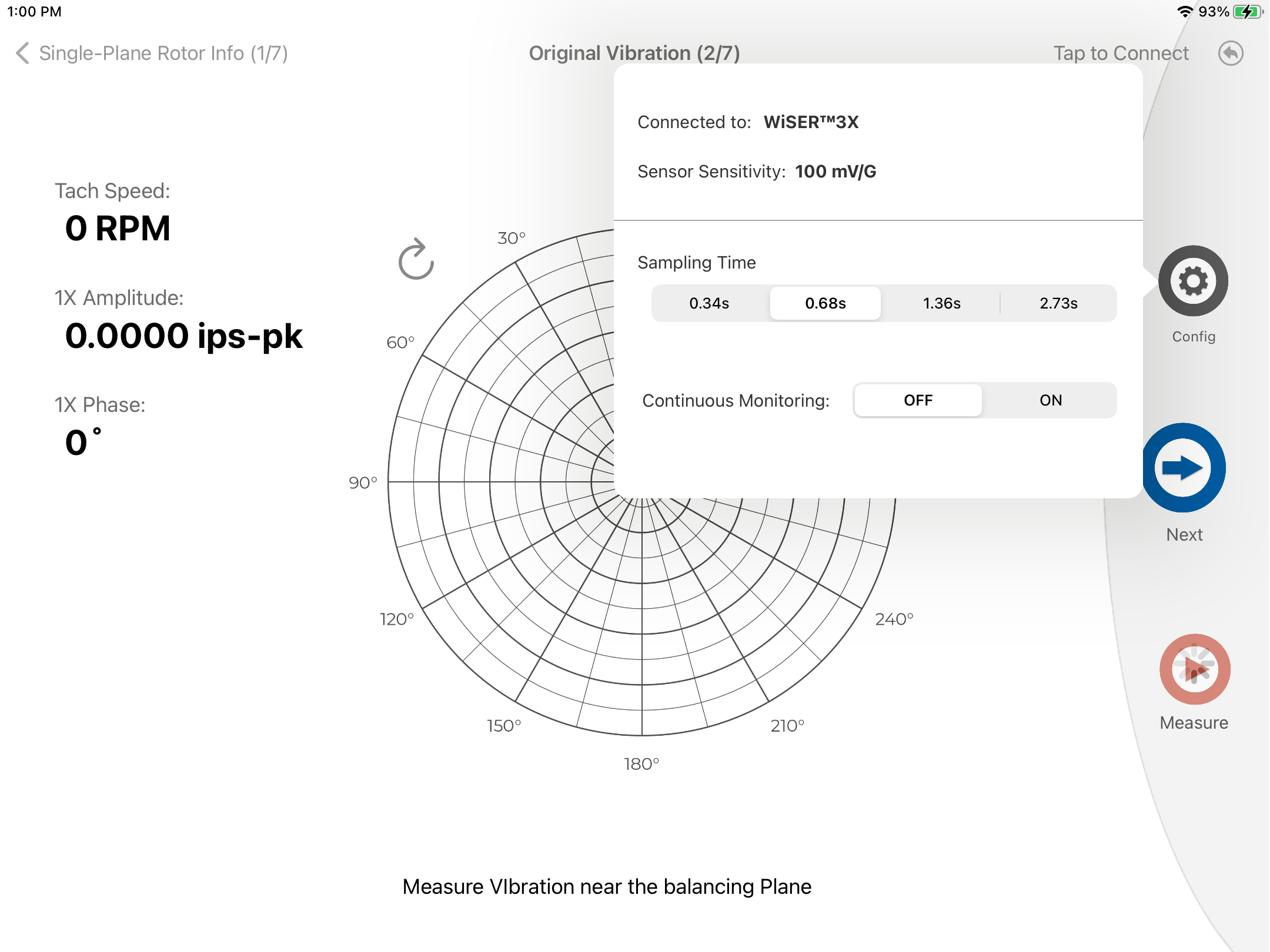
- The user can change the sensor sampling setting by opening the "Settings" pop-up as shown below. This setting was automatically selected from the initial rotor parameters. The user can also change to continuous mode to get a live display of the vibration vector on the polar plot. Other settings such as units and filters can be changed in the main Configuration view.
- Once the sensor displays the connected status on the top bar menu, Click on the Measure ▶︎ button to collect the vibration vector, which will also show in the polar plot with a circle and a number 1. The green circle in the polar plot indicates the threshold (defined on the first screen). The RPM, amplitude and phase will display on a side.
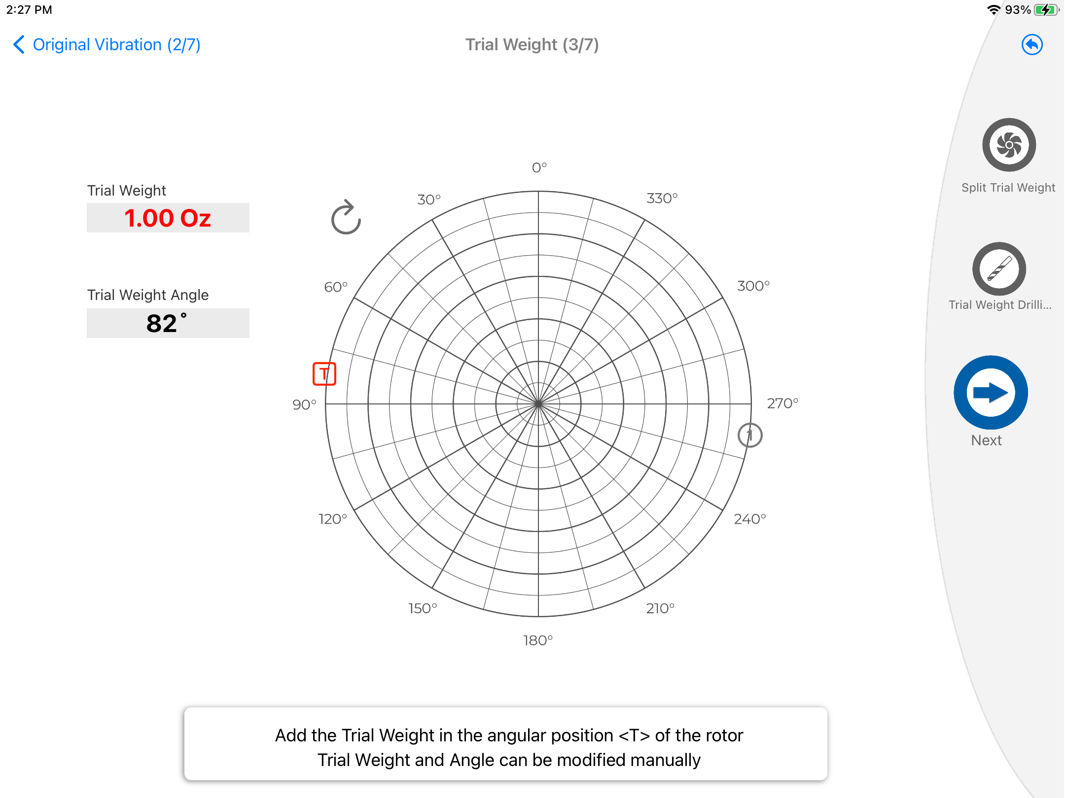
- The next screen (3 of 7)will display the angular location and amount of trial weight to be mounted on the rotor. The user can change the trial value or the angle by tapping on each field. Once a value is changed, it will be displayed in red color. The Trial weight location will be displayed on the polar plot with a red box and the letter "T". Mount the trial weight on the rotor on the same final location and magnitude as shown in the polar plot.
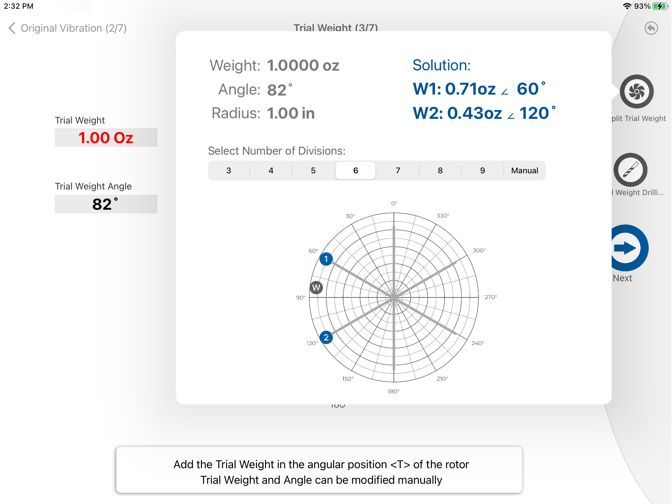
- In the case the trial weight does not match an available position in the rotor to be mounted, the user can open the "Split Weight" pop-up assistant and select the number of available angular positions to get a split value for the weight.
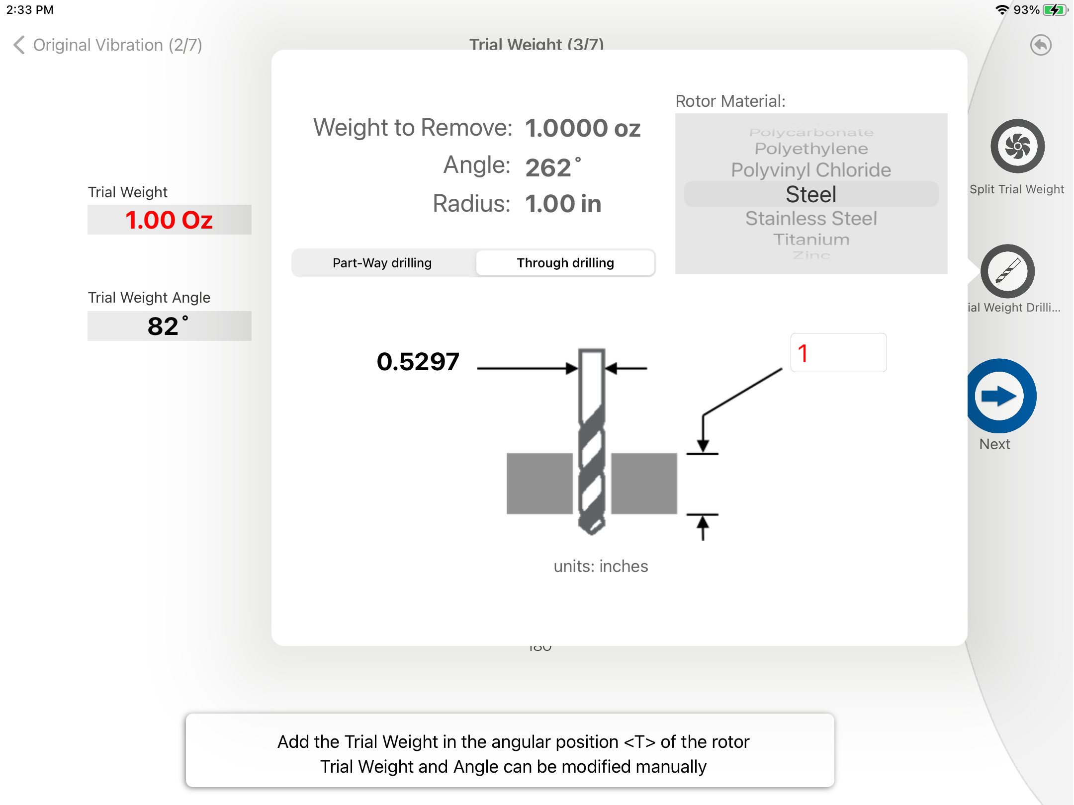
- In the case the trial weight must be removed, instead of added, the user can open the "Drill" assistant pop-up and select the material, and in the case the hole is a part-way drilling enter the drill diameter to obtain the hole depth; in the case of a through drilling the user must enter the material depth to get the drill diameter to be used.
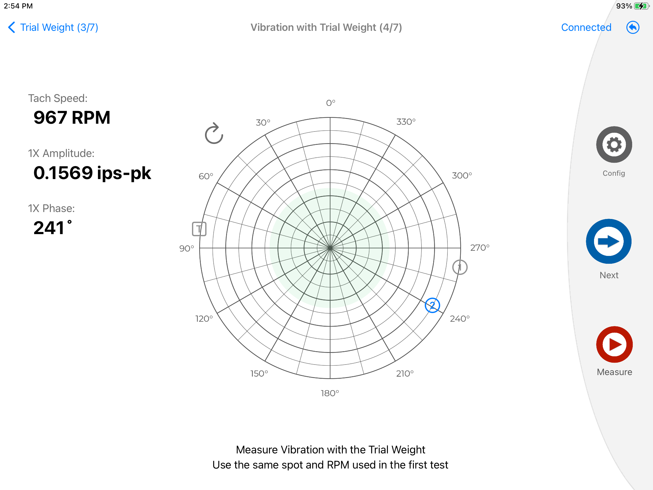
- The next screen (4 of 7) will require the user to take a new reading of the vibration vector with the trial weight on the rotor. Press the "Measure" button to acquire the data. The new amplitude and angular position of the 1X filtered vibration will be displayed and shown in the polar plot with a blue circle "2".
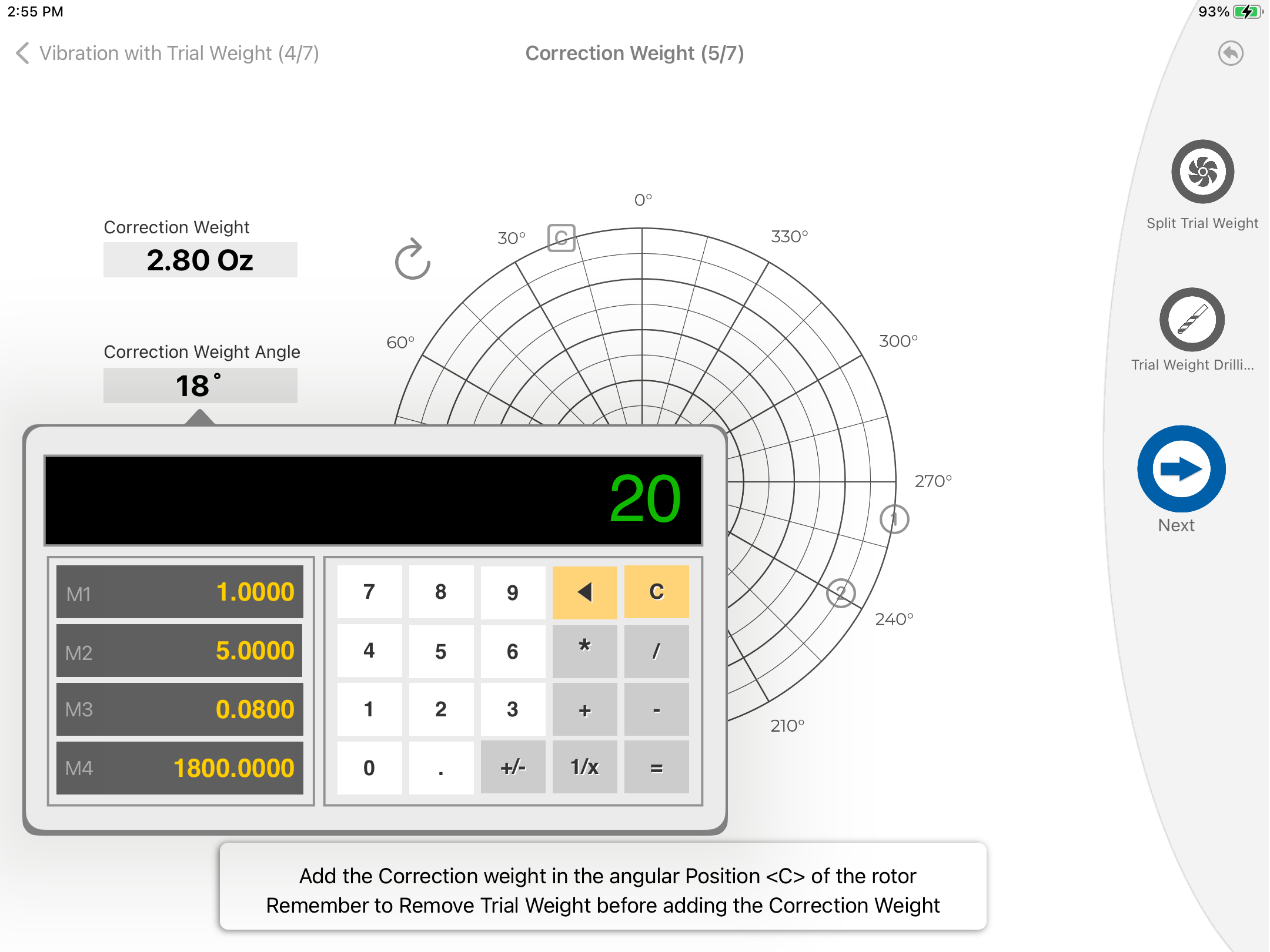
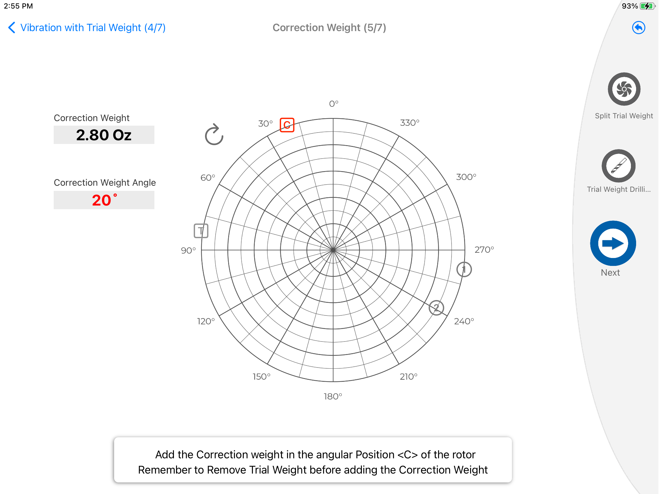
- The next screen (5 of 7) will calculate the correction weight to be mounted on the rotor and will be displayed in the polar plot with a red square "C". The user can manually change the angular position and weight magnitude here.
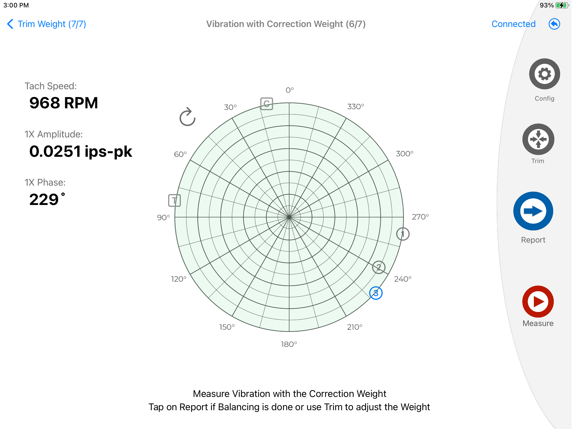
- After mounting the correction weight, click next (to open view 6 of 7) and measure again the vibration by pressing the "Measure" button. The measured 1X Filtered Vibration value with the correction weight is below the threshold value (green zone in the polar plot). Pressing the "Report" button will open the pdf report, but the user has the option to perform a trim balancing.
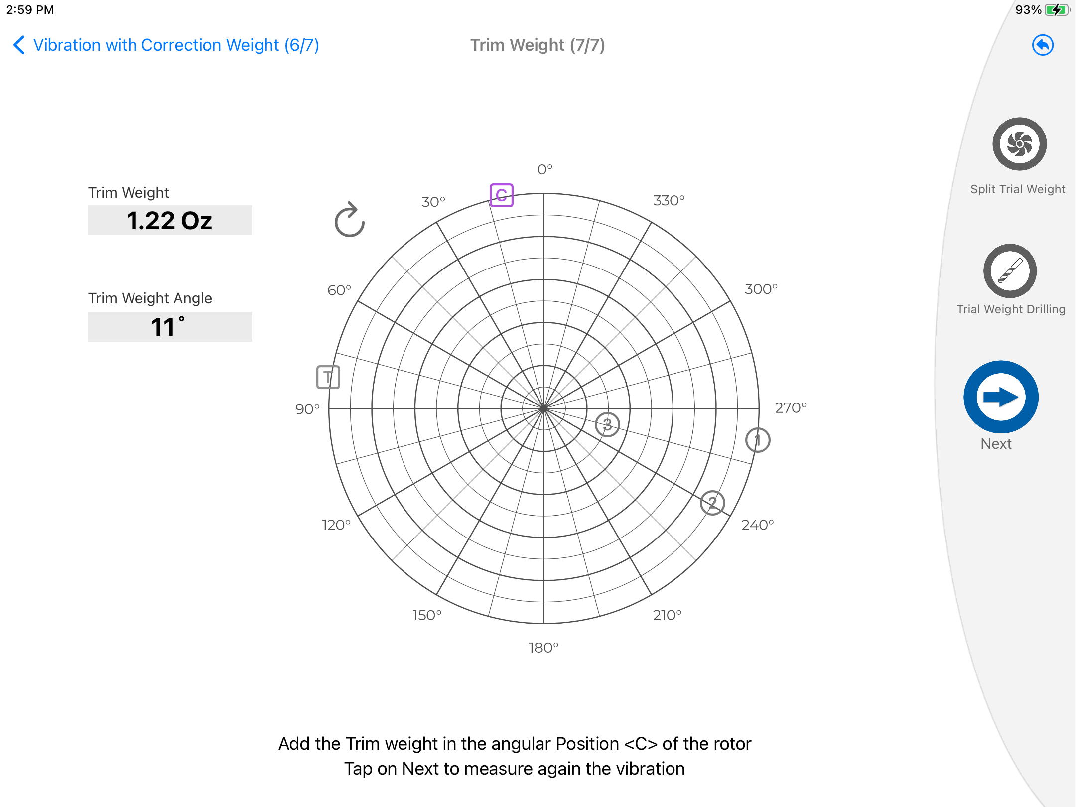
- Pressing the "Trim" button will calculate a new trim correction weight, as shown below. Place the trim weight on the rotor.
- Click "Next" and measure again the vibration. To perform more trimming click on "Trim" and to end the process and generate the pdf report, click on the "Report" button.
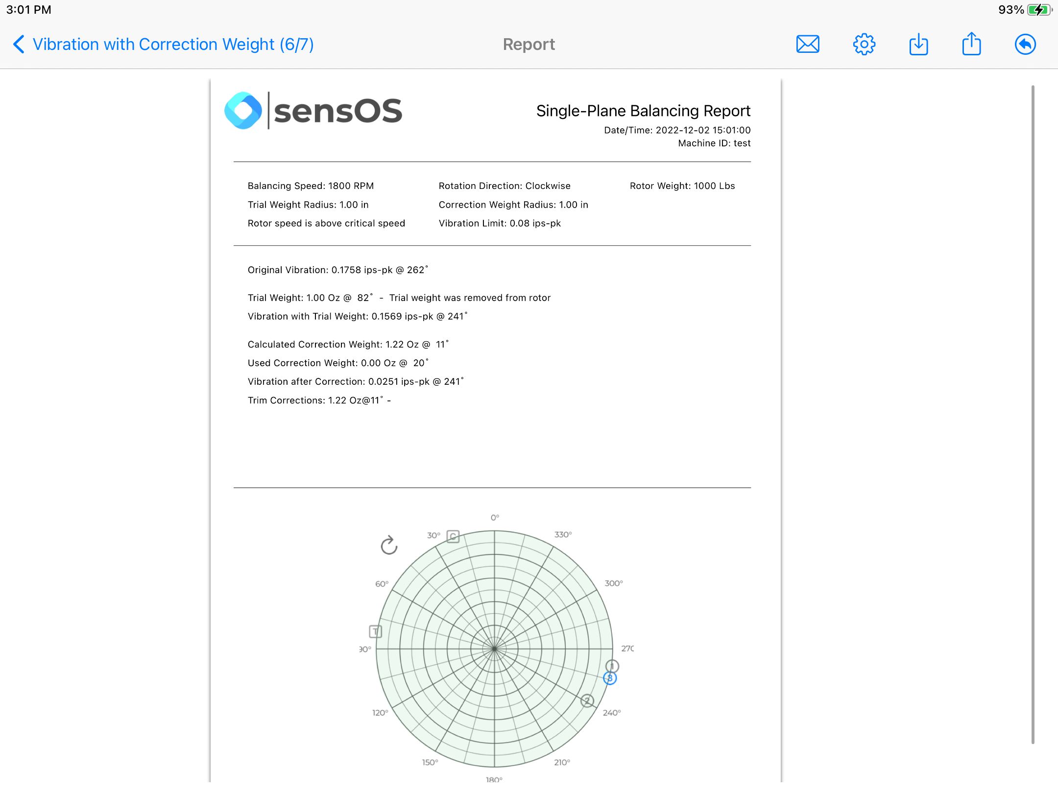
- The report will display all the measurements, weights added, trims and the final polar plot. User can go back to the initial screen by clicking on the return ⤴️ on the top bar menu. The report can be sent, printed, modified, saved locally or to the cloud bucket, see more details in Generating a pdf Report
Note: The user can navigate to the previous screen or to the next screen at any time without loosing any data.

Note: Pressing the ⤴️ button in the top bar menu on any screen will take the user back to the initial screen.
Configuration
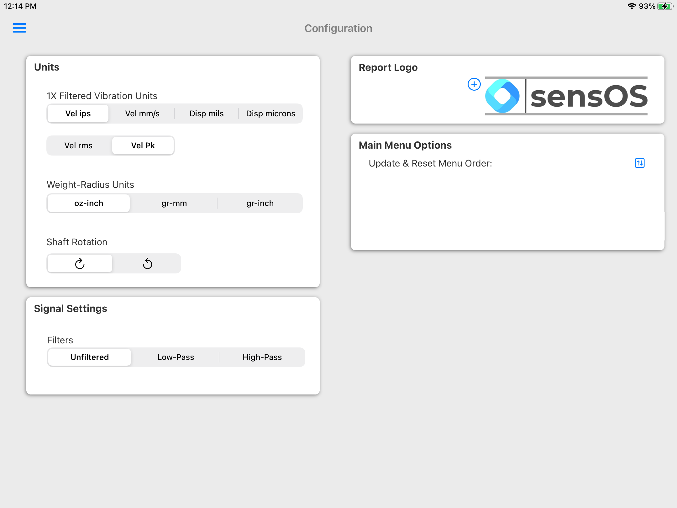
- From the Main menu, click the top left menu button to open the left drawer with more options. Select 'Configuration' from the left menu
- In the main configuration the user can change the default units, integration type, shaft rotation direction and filters. The user can also add here a default logo for the reports.
For devices using the audio input and iPadOS version above 18, the Audio Hardware Quality selector should be set to "High"
Report
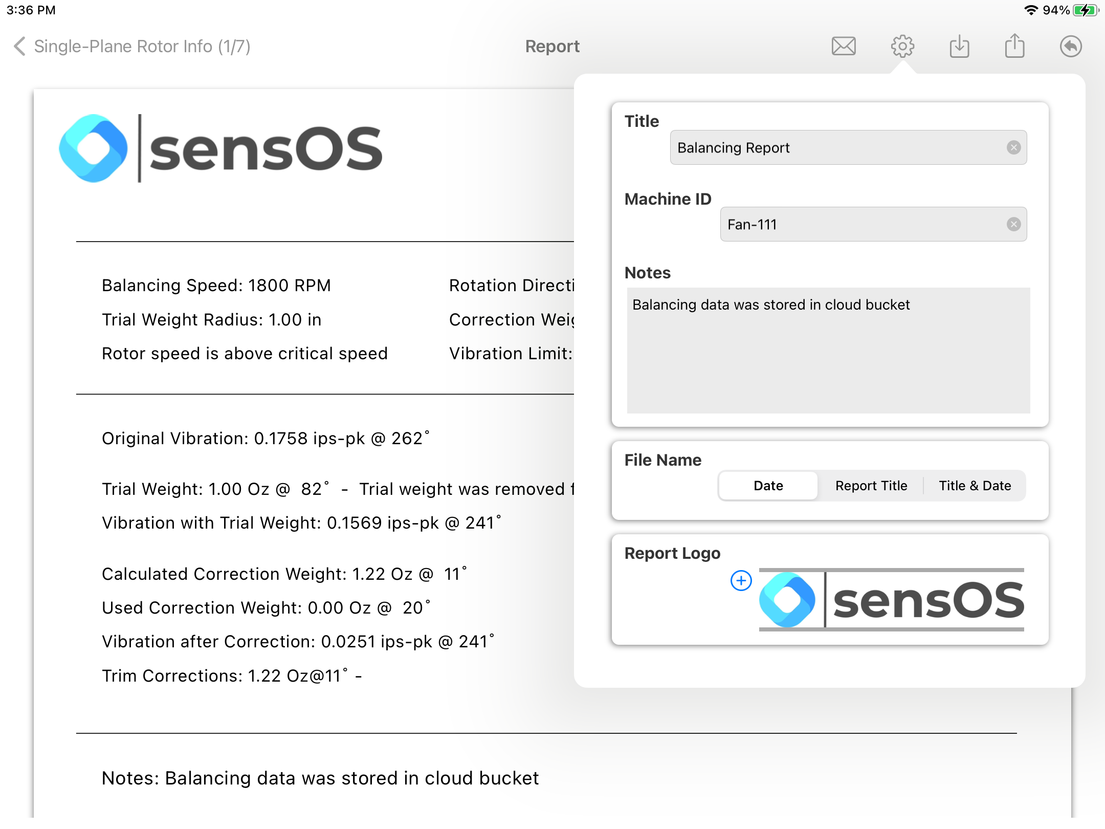
- Clicking on the Report button will open a new view with the pdf report. The report view contains several options in the top bar menu: 1:Send by Email, 2:Configuration, 3:Save pdf locally, 4:Upload Report to the user's Cloud bucket, 5:Return to the initial screen
- The Report Configuration pop-up allows the user to enter the Report Title, Machine ID and Notes to be added to the report. Here the user can also select a logo for the report. The report file name be default is the actual date and time, but the user can change it to the title name of the report or to both, the title name and date.
Files & Data
- By selecting the Files & Data button in the top bar, the user can save/load the balancing data locally, in the cloud bucket or in the cloud hierarchy tree.
- To save data locally, select the 'Local' option in the first selector and then select 'Save' in the selector below. By default the name of the file will be the timestamp, but the user can customize it here and click on the blue save button on the right.
- To load data locally, select the 'Local' option in the first selector and then select 'Load' in the selector below. A list of all available local files will appear, tap on the desired file and it will load the data in the actual balancing.
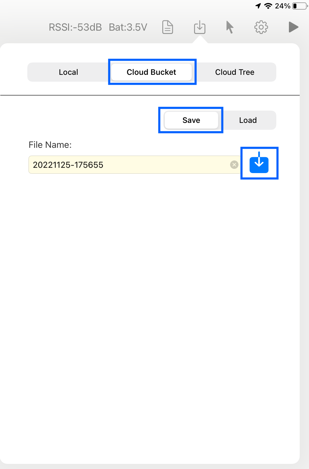
- To save data on the user's cloud bucket, select the 'Cloud Bucket' option in the first selector and then select 'Save' in the selector below. By default the name of the file will be the timestamp, but the user can customize it here and click on the blue save button on the right, this will upload the data file to the user's cloud bucket.
- To load data from the user's cloud bucket, select the 'Cloud Bucket' option in the first selector and then select 'Load' in the selector below. A list of all available local files will appear, tap on the desired file and it will load the data in the actual balancing.
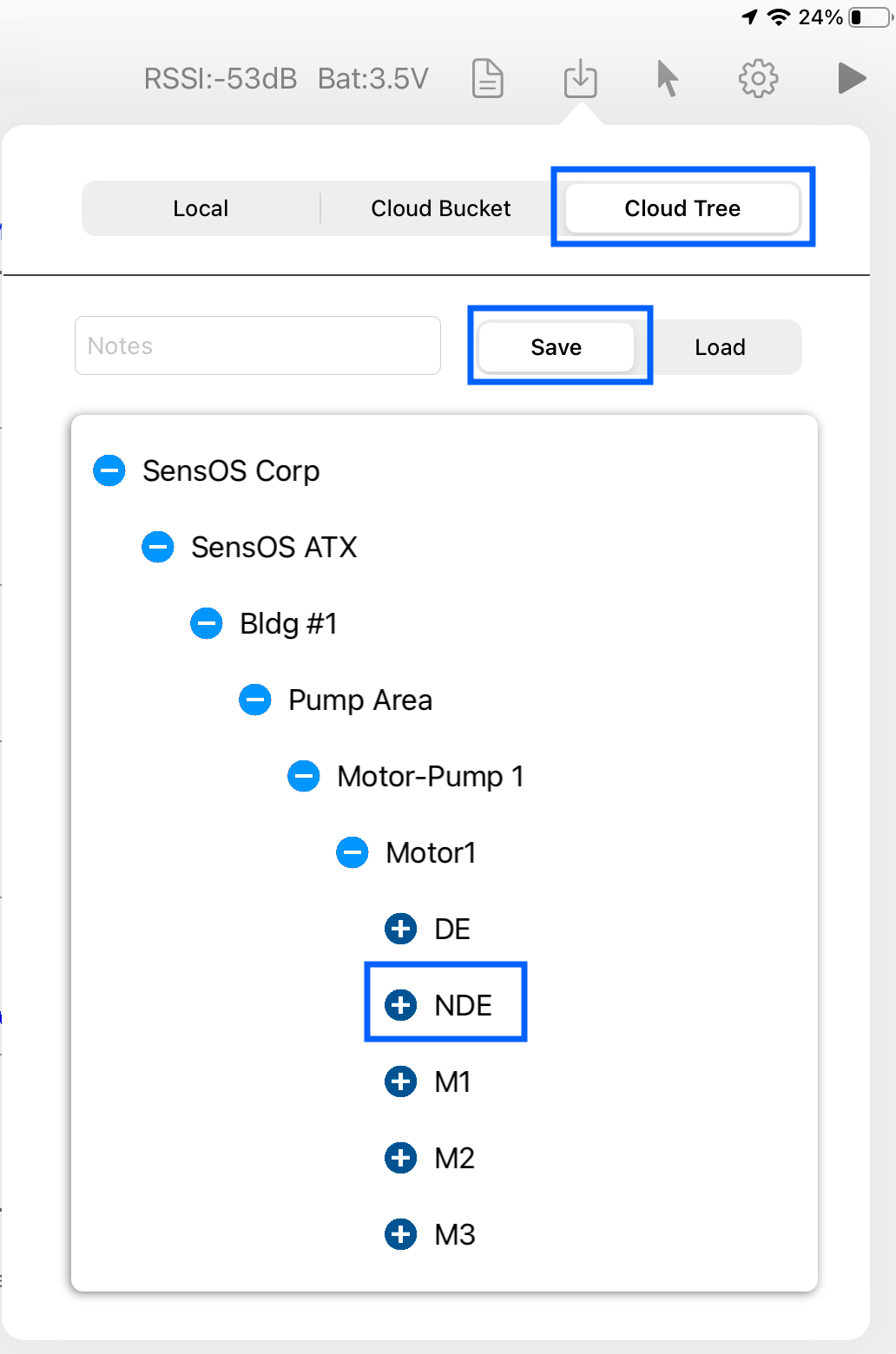
- To save data on the user's hierarchy tree, select the 'Cloud Tree' option in the first selector and then select 'Save' in the selector below. The user's hierarchy tree will appear, navigate to the point to save the data by clicking on each location, machine, component, and point.
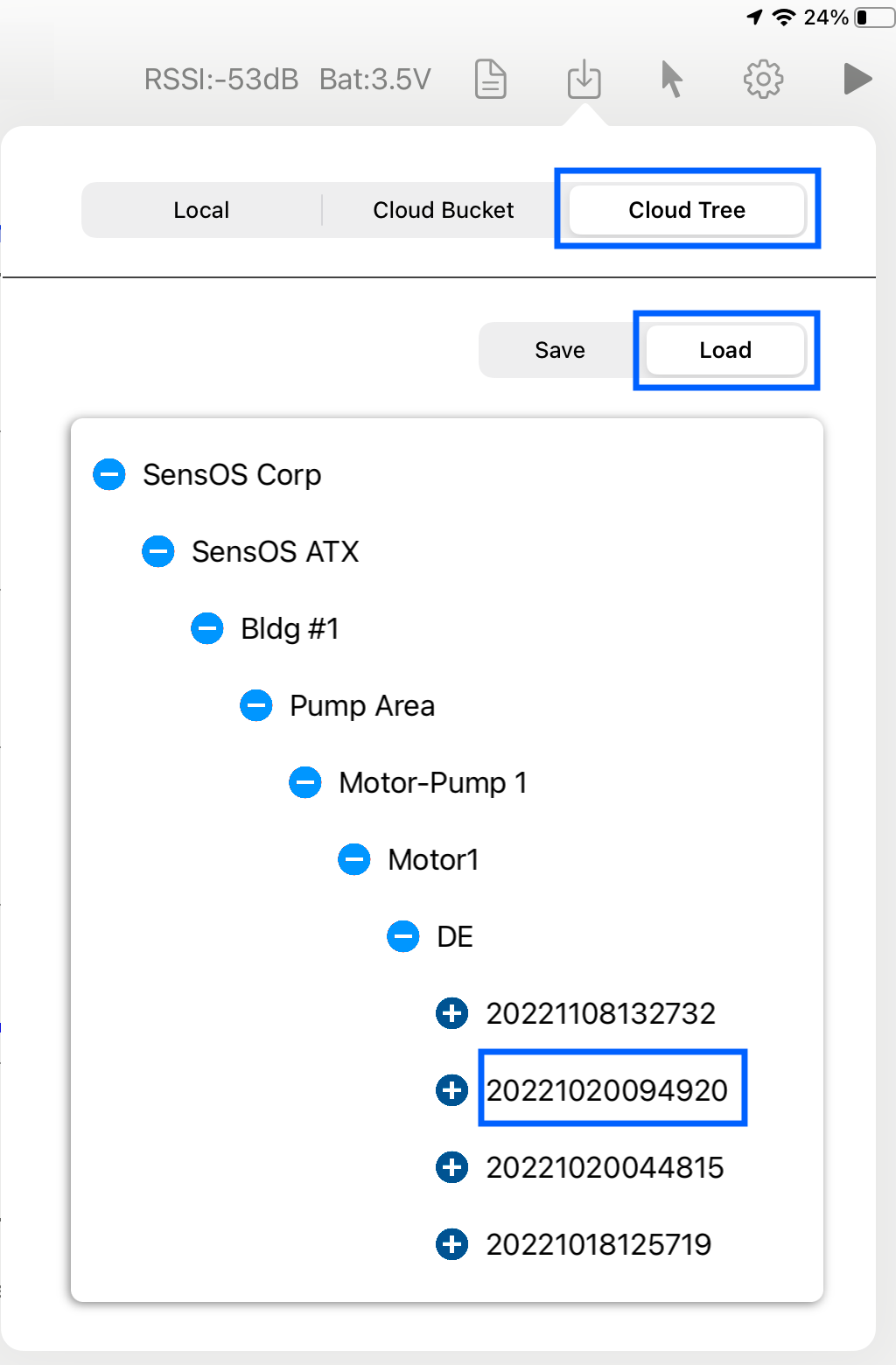
- To load data from the user's hierarchy tree, select the 'Cloud Tree' option in the first selector and then select 'Load' in the selector below. The user's hierarchy tree will appear, navigate to the desired reading (timestamp) by clicking on the desired locations, machine, component and point.


Changelog
See what's new added, changed, fixed, improved or updated in the latest versions.
Version 1.13 b.46 (22 Nov, 2022)
- Optimized Optimized for iPadOS 16
Version 1.01 b.23 (05 Oct, 2021)
Initial Release